quantitative research paper in environmental science

Thank you for visiting nature.com. You are using a browser version with limited support for CSS. To obtain the best experience, we recommend you use a more up to date browser (or turn off compatibility mode in Internet Explorer). In the meantime, to ensure continued support, we are displaying the site without styles and JavaScript.

• View all journals
• My Account Login
• Explore content
• About the journal
• Publish with us
• Sign up for alerts
• Open access
• Published: 06 May 2020

Deforestation and world population sustainability: a quantitative analysis

• Mauro Bologna 1   na1 &
• Gerardo Aquino 2 , 3 , 4   na1  

Scientific Reports volume  10 , Article number:  7631 ( 2020 ) Cite this article

199k Accesses

66 Citations

1359 Altmetric

Metrics details

• Applied mathematics
• Environmental impact
• Population dynamics
• Statistical physics, thermodynamics and nonlinear dynamics

In this paper we afford a quantitative analysis of the sustainability of current world population growth in relation to the parallel deforestation process adopting a statistical point of view. We consider a simplified model based on a stochastic growth process driven by a continuous time random walk, which depicts the technological evolution of human kind, in conjunction with a deterministic generalised logistic model for humans-forest interaction and we evaluate the probability of avoiding the self-destruction of our civilisation. Based on the current resource consumption rates and best estimate of technological rate growth our study shows that we have very low probability, less than 10% in most optimistic estimate, to survive without facing a catastrophic collapse.

Similar content being viewed by others

The qualified prevalence of natural and planted tropical reforestation

Deforestation reduces rainfall and agricultural revenues in the Brazilian Amazon

Deforestation in Colombian protected areas increased during post-conflict periods

Introduction.

In the last few decades, the debate on climate change has assumed global importance with consequences on national and global policies. Many factors due to human activity are considered as possible responsible of the observed changes: among these water and air contamination (mostly greenhouse effect) and deforestation are the mostly cited. While the extent of human contribution to the greenhouse effect and temperature changes is still a matter of discussion, the deforestation is an undeniable fact. Indeed before the development of human civilisations, our planet was covered by 60 million square kilometres of forest 1 . As a result of deforestation, less than 40 million square kilometres currently remain 2 . In this paper, we focus on the consequence of indiscriminate deforestation.

Trees’ services to our planet range from carbon storage, oxygen production to soil conservation and water cycle regulation. They support natural and human food systems and provide homes for countless species, including us, through building materials. Trees and forests are our best atmosphere cleaners and, due to the key role they play in the terrestrial ecosystem, it is highly unlikely to imagine the survival of many species, including ours, on Earth without them. In this sense, the debate on climate change will be almost obsolete in case of a global deforestation of the planet. Starting from this almost obvious observation, we investigate the problem of the survival of humanity from a statistical point of view. We model the interaction between forests and humans based on a deterministic logistic-like dynamics, while we assume a stochastic model for the technological development of the human civilisation. The former model has already been applied in similar contexts 3 , 4 while the latter is based on data and model of global energy consumption 5 , 6 used as a proxy for the technological development of a society. This gives solidity to our discussion and we show that, keeping the current rate of deforestation, statistically the probability to survive without facing a catastrophic collapse, is very low. We connect such probability to survive to the capability of humankind to spread and exploit the resources of the full solar system. According to Kardashev scale 7 , 8 , which measures a civilisation’s level of technological advancement based on the amount of energy they are able to use, in order to spread through the solar system we need to be able to harness the energy radiated by the Sun at a rate of ≈4 × 10 26 Watt. Our current energy consumption rate is estimated in ≈10 13 Watt 9 . As showed in the subsections “Statistical Model of technological development” and “Numerical results” of the following section, a successful outcome has a well defined threshold and we conclude that the probability of avoiding a catastrophic collapse is very low, less than 10% in the most optimistic estimate.

Model and Results

Deforestation.

The deforestation of the planet is a fact 2 . Between 2000 and 2012, 2.3 million Km 2 of forests around the world were cut down 10 which amounts to 2 × 10 5 Km 2 per year. At this rate all the forests would disappear approximatively in 100–200 years. Clearly it is unrealistic to imagine that the human society would start to be affected by the deforestation only when the last tree would be cut down. The progressive degradation of the environment due to deforestation would heavily affect human society and consequently the human collapse would start much earlier.

Curiously enough, the current situation of our planet has a lot in common with the deforestation of Easter Island as described in 3 . We therefore use the model introduced in that reference to roughly describe the humans-forest interaction. Admittedly, we are not aiming here for an exact exhaustive model. It is probably impossible to build such a model. What we propose and illustrate in the following sections, is a simplified model which nonetheless allows us to extrapolate the time scales of the processes involved: i.e. the deterministic process describing human population and resource (forest) consumption and the stochastic process defining the economic and technological growth of societies. Adopting the model in 3 (see also 11 ) we have for the humans-forest dynamics

where N represent the world population and R the Earth surface covered by forest. β is a positive constant related to the carrying capacity of the planet for human population, r is the growth rate for humans (estimated as r  ~ 0.01 years −1 ) 12 , a 0 may be identified as the technological parameter measuring the rate at which humans can extract the resources from the environment, as a consequence of their reached technological level. r ’ is the renewability parameter representing the capability of the resources to regenerate, (estimated as r ’ ~ 0.001 years −1 ) 13 , R c the resources carrying capacity that in our case may be identified with the initial 60 million square kilometres of forest. A closer look at this simplified model and at the analogy with Easter Island on which is based, shows nonetheless, strong similarities with our current situation. Like the old inhabitants of Easter Island we too, at least for few more decades, cannot leave the planet. The consumption of the natural resources, in particular the forests, is in competition with our technological level. Higher technological level leads to growing population and higher forest consumption (larger a 0 ) but also to a more effective use of resources. With higher technological level we can in principle develop technical solutions to avoid/prevent the ecological collapse of our planet or, as last chance, to rebuild a civilisation in the extraterrestrial space (see section on the Fermi paradox). The dynamics of our model for humans-forest interaction in Eqs. ( 1 , 2 ), is typically characterised by a growing human population until a maximum is reached after which a rapid disastrous collapse in population occurs before eventually reaching a low population steady state or total extinction. We will use this maximum as a reference for reaching a disastrous condition. We call this point in time the “no-return point” because if the deforestation rate is not changed before this time the human population will not be able to sustain itself and a disastrous collapse or even extinction will occur. As a first approximation 3 , since the capability of the resources to regenerate, r ′, is an order of magnitude smaller than the growing rate for humans, r , we may neglect the first term in the right hand-side of Eq. ( 2 ). Therefore, working in a regime of the exploitation of the resources governed essentially by the deforestation, from Eq. ( 2 ) we can derive the rate of tree extinction as

The actual population of the Earth is N  ~ 7.5 × 10 9 inhabitants with a maximum carrying capacity estimated 14 of N c  ~ 10 10 inhabitants. The forest carrying capacity may be taken as 1 R c  ~ 6 × 10 7 Km 2 while the actual surface of forest is \(R\lesssim 4\times {10}^{7}\) Km 2 . Assuming that β is constant, we may estimate this parameter evaluating the equality N c ( t ) =  βR ( t ) at the time when the forests were intact. Here N c ( t ) is the instantaneous human carrying capacity given by Eq. ( 1 ). We obtain β  ~  N c / R c  ~ 170.

In alternative we may evaluate β using actual data of the population growth 15 and inserting it in Eq. ( 1 ). In this case we obtain a range \(700\lesssim \beta \lesssim 900\) that gives a slightly favourable scenario for the human kind (see below and Fig.  4 ). We stress anyway that this second scenario depends on many factors not least the fact that the period examined in 15 is relatively short. On the contrary β  ~ 170 is based on the accepted value for the maximum human carrying capacity. With respect to the value of parameter a 0 , adopting the data relative to years 2000–2012 of ref. 10 ,we have

The time evolution of system ( 1 ) and ( 2 ) is plotted in Figs.  1 and 2 . We note that in Fig.  1 the numerical value of the maximum of the function N ( t ) is N M  ~ 10 10 estimated as the carrying capacity for the Earth population 14 . Again we have to stress that it is unrealistic to think that the decline of the population in a situation of strong environmental degradation would be a non-chaotic and well-ordered decline, that is also way we take the maximum in population and the time at which occurs as the point of reference for the occurrence of an irreversible catastrophic collapse, namely a ‘no-return’ point.

On the left: plot of the solution of Eq. ( 1 ) with the initial condition N 0  = 6 × 10 9 at initial time t  = 2000 A.C. On the right: plot of the solution of Eq. ( 2 ) with the initial condition R 0  = 4 × 10 7 . Here β  = 700 and a 0  = 10 −12 .

On the left: plot of the solution of Eq. ( 1 ) with the initial condition N 0  = 6 × 10 9 at initial time t  = 2000 A.C. On the right: plot of the solution of Eq. ( 2 ) with the initial condition R 0  = 4 × 10 7 . Here β  = 170 and a 0  = 10 −12 .

Statistical model of technological development

According to Kardashev scale 7 , 8 , in order to be able to spread through the solar system, a civilisation must be capable to build a Dyson sphere 16 , i.e. a maximal technological exploitation of most the energy from its local star, which in the case of the Earth with the Sun would correspond to an energy consumption of E D  ≈ 4 × 10 26 Watts, we call this value Dyson limit. Our actual energy consumption is estimated in E c  ≈ 10 13 Watts (Statistical Review of World Energy source) 9 . To describe our technological evolution, we may roughly schematise the development as a dichotomous random process

where T is the level of technological development of human civilisation that we can also identify with the energy consumption. α is a constant parameter describing the technological growth rate (i.e. of T ) and ξ ( t ) a random variable with values 0, 1. We consider therefore, based on data of global energy consumption 5 , 6 an exponential growth with fluctuations mainly reflecting changes in global economy. We therefore consider a modulated exponential growth process where the fluctuations in the growth rate are captured by the variable ξ ( t ). This variable switches between values 0, 1 with waiting times between switches distributed with density ψ ( t ). When ξ ( t ) = 0 the growth stops and resumes when ξ switches to ξ ( t ) = 1. If we consider T more strictly as describing the technological development, ξ ( t ) reflects the fact that investments in research can have interruptions as a consequence of alternation of periods of economic growth and crisis. With the following transformation,

differentiating both sides respect to t and using Eq. ( 5 ), we obtain for the transformed variable W

where \(\bar{\xi }(t)=2[\xi (t)-\langle \xi \rangle ]\) and 〈ξ 〉 is the average of ξ ( t ) so that \(\bar{\xi }(t)\) takes the values ±1.

The above equation has been intensively studied, and a general solution for the probability distribution P ( W , t ) generated by a generic waiting time distribution can be found in literature 17 . Knowing the distribution we may evaluate the first passage time distribution in reaching the necessary level of technology to e.g. live in the extraterrestrial space or develop any other way to sustain population of the planet. This characteristic time has to be compared with the time that it will take to reach the no-return point. Knowing the first passage time distribution 18 we will be able to evaluate the probability to survive for our civilisation.

If the dichotomous process is a Poissonian process with rate γ then the correlation function is an exponential, i.e.

and Eq. ( 7 ) generates for the probability density the well known telegrapher’s equation

We note that the approach that we are following is based on the assumption that at random times, exponentially distributed with rate γ , the dichotomous variable \(\bar{\xi }\) changes its value. With this assumption the solution to Eq. ( 9 ) is

where I n ( z ) are the modified Bessel function of the first kind. Transforming back to the variable T we have

where for sake of compactness we set

In Laplace transform we have

The first passage time distribution, in laplace transform, is evaluated as 19

Inverting the Laplace transform we obtain

which is confirmed (see Fig.  3 ) by numerical simulations. The time average to get the point x for the first time is given by

which interestingly is double the time it would take if a pure exponential growth occurred, depends on the ratio between final and initial value of T and is independent of γ . We also stress that this result depends on parameters directly related to the stage of development of the considered civilisation, namely the starting value T 1 , that we assume to be the energy consumption E c of the fully industrialised stage of the civilisation evolution and the final value T , that we assume to be the Dyson limit E D , and the technological growth rate α . For the latter we may, rather optimistically, choose the value α  = 0.345, following the Moore Law 20 (see next section). Using the data above, relative to our planet’s scenario, we obtain the estimate of 〈 t 〉 ≈ 180 years. From Figs.  1 and 2 we see that the estimate for the no-return time are 130 and 22 years for β  = 700 and β  = 170 respectively, with the latter being the most realistic value. In either case, these estimates based on average values, being less than 180 years, already portend not a favourable outcome for avoiding a catastrophic collapse. Nonetheless, in order to estimate the actual probability for avoiding collapse we cannot rely on average values, but we need to evaluate the single trajectories, and count the ones that manage to reach the Dyson limit before the ‘no-return point’. We implement this numerically as explained in the following.

(Left) Comparison between theoretical prediction of Eq. ( 15 ) (black curve) and numerical simulation of Eq. ( 3 ) (cyan curve) for γ  = 4 (arbitrary units). (Right) Comparison between theoretical prediction of Eq. ( 15 ) (red curve) and numerical simulation of Eq. ( 3 ) (black curve) for γ  = 1/4 (arbitrary units).

(Left panel) Probability p suc of reaching Dyson value before reaching “no-return” point as function of α and a for β  = 170. Parameter a is expressed in Km 2 ys −1 . (Right panel) 2D plot of p suc for a  = 1.5 × 10 −4 Km 2 ys −1 as a function of α . Red line is p suc for β  = 170. Black continuous lines (indistinguishable) are p suc for β  = 300 and 700 respectively (see also Fig.  6 ). Green dashed line indicates the value of α corresponding to Moore’s law.

Numerical results

We run simulations of Eqs. ( 1 ), ( 2 ) and ( 5 ) simultaneously for different values of of parameters a 0 and α for fixed β and we count the number of trajectories that reach Dyson limit before the population level reaches the “no-return point” after which rapid collapse occurs. More precisely, the evolution of T is stochastic due to the dichotomous random process ξ ( t ), so we generate the T ( t ) trajectories and at the same time we follow the evolution of the population and forest density dictated by the dynamics of Eqs. ( 1 ), ( 2 ) 3 until the latter dynamics reaches the no-return point (maximum in population followed by collapse). When this happens, if the trajectory in T ( t ) has reached the Dyson limit we count it as a success, otherwise as failure. This way we determine the probabilities and relative mean times in Figs.  5 , 6 and 7 . Adopting a weak sustainability point of view our model does not specify the technological mechanism by which the successful trajectories are able to find an alternative to forests and avoid collapse, we leave this undefined and link it exclusively and probabilistically to the attainment of the Dyson limit. It is important to notice that we link the technological growth process described by Eq. ( 5 ) to the economic growth and therefore we consider, for both economic and technological growth, a random sequence of growth and stagnation cycles, with mean periods of about 1 and 4 years in accordance with estimates for the driving world economy, i.e. the United States according to the National Bureau of Economic Research 21 .

Average time τ (in years) to reach Dyson value before hitting “no-return” point (success, left) and without meeting Dyson value (failure, right) as function of α and a for β  = 170. Plateau region (left panel) where τ  ≥ 50 corresponds to diverging τ , i.e. Dyson value not being reached before hitting “no-return” point and therefore failure. Plateau region at τ  = 0 (right panel), corresponds to failure not occurring, i.e. success. Parameter a is expressed in Km 2 ys −1 .

Probability p suc of reaching Dyson value before hitting “no-return” point as function of α and a for β  = 300 (left) and 700 (right). Parameter a is expressed in Km 2 ys −1 .

Probability of reaching Dyson value p suc before reaching “no-return” point as function of β and α for a  = 1.5 × 10 −4 Km 2 ys −1 .

In Eq. ( 1 , 2 ) we redefine the variables as N ′ =  N / R W and R ′ =  R / R W with \({R}_{W}\simeq 150\times {10}^{6}\,K{m}^{2}\) the total continental area, and replace parameter a 0 accordingly with a  =  a 0  ×  R W  = 1.5 × 10 −4 Km 2 ys −1 . We run simulations accordingly starting from values \({R{\prime} }_{0}\) and \({N{\prime} }_{0}\) , based respectively on the current forest surface and human population. We take values of a from 10 −5 to 3 × 10 −4 Km 2 ys −1 and for α from 0.01 ys −1 to 4.4 ys −1 . Results are shown in Figs.  4 and 6 . Figure  4 shows a threshold value for the parameter α , the technological growth rate, above which there is a non-zero probability of success. This threshold value increases with the value of the other parameter a . As shown in Fig.  7 this values depends as well on the value of β and higher values of β correspond to a more favourable scenario where the transition to a non-zero probability of success occurs for smaller α , i.e. for smaller, more accessible values, of technological growth rate. More specifically, left panel of Fig.  4 shows that, for the more realistic value β  = 170, a region of parameter values with non-zero probability of avoiding collapse corresponds to values of α larger than 0.5. Even assuming that the technological growth rate be comparable to the value α  = log(2)/2 = 0.345 ys −1 , given by the Moore Law (corresponding to a doubling in size every two years), therefore, it is unlikely in this regime to avoid reaching the the catastrophic ‘no-return point’. When the realistic value of a  = 1.5 × 10 4 Km 2 ys −1 estimated from Eq. ( 4 ), is adopted, in fact, a probability less than 10% is obtained for avoiding collapse with a Moore growth rate, even when adopting the more optimistic scenario corresponding to β  = 700 (black curve in right panel of Fig.  4 ). While an α larger than 1.5 is needed to have a non-zero probability of avoiding collapse when β  = 170 (red curve, same panel). As far as time scales are concerned, right panel of Fig.  5 shows for β  = 170 that even in the range α  > 0.5, corresponding to a non-zero probability of avoiding collapse, collapse is still possible, and when this occurs, the average time to the ‘no-return point’ ranges from 20 to 40 years. Left panel in same figure, shows for the same parameters, that in order to avoid catastrophe, our society has to reach the Dyson’s limit in the same average amount of time of 20–40 years.

In Fig.  7 we show the dependence of the model on the parameter β for a  = 1.5 × 10 −4 .

We run simulations of Eqs. ( 1 ), ( 2 ) and ( 5 ) simultaneously for different values of of parameters a 0 and α depending on β as explained in Methods and Results to generate Figs.  5 , 6 and 7 . Equations ( 1 ), ( 2 ) are integrated via standard Euler method. Eq. ( 5 ) is integrated as well via standard Euler method between the random changes of the variable ξ . The stochastic dichotomous process ξ is generated numerically in the following way: using the random number generator from gsl library we generate the times intervals between the changes of the dichotomous variable ξ  = 0, 1, with an exponential distribution(with mean values of 1 and 4 years respectively), we therefore obtain a time series of 0 and 1 for each trajectory. We then integrate Eq. ( 5 ) in time using this time series and we average over N  = 10000 trajectories. The latter procedure is used to carry out simulations in Figs.  3 and 4 as well in order to evaluate the first passage time probabilities. All simulations are implemented in C++.

Fermi paradox

In this section we briefly discuss a few considerations about the so called Fermi paradox that can be drawn from our model. We may in fact relate the Fermi paradox to the problem of resource consumption and self destruction of a civilisation. The origin of Fermi paradox dates back to a casual conversation about extraterrestrial life that Enrico Fermi had with E. Konopinski, E. Teller and H. York in 1950, during which Fermi asked the famous question: “where is everybody?”, since then become eponymous for the paradox. Starting from the closely related Drake equation 22 , 23 , used to estimate the number of extraterrestrial civilisations in the Milky Way, the debate around this topic has been particularly intense in the past (for a more comprehensive covering we refer to Hart 24 , Freitas 25 and reference therein). Hart’s conclusion is that there are no other advanced or ‘technological’ civilisations in our galaxy as also supported recently by 26 based on a careful reexamination of Drake’s equation. In other words the terrestrial civilisation should be the only one living in the Milk Way. Such conclusions are still debated, but many of Hart’s arguments are undoubtedly still valid while some of them need to be rediscussed or updated. For example, there is also the possibility that avoiding communication might actually be an ‘intelligent’ choice and a possible explanation of the paradox. On several public occasions, in fact, Professor Stephen Hawking suggested human kind should be very cautious about making contact with extraterrestrial life. More precisely when questioned about planet Gliese 832c’s potential for alien life he once said: “One day, we might receive a signal from a planet like this, but we should be wary of answering back”. Human history has in fact been punctuated by clashes between different civilisations and cultures which should serve as caveat. From the relatively soft replacement between Neanderthals and Homo Sapiens (Kolodny 27 ) up to the violent confrontation between native Americans and Europeans, the historical examples of clashes and extinctions of cultures and civilisations have been quite numerous. Looking at human history Hawking’s suggestion appears as a wise warning and we cannot role out the possibility that extraterrestrial societies are following similar advice coming from their best minds.

With the help of new technologies capable of observing extrasolar planetary systems, searching and contacting alien life is becoming a concrete possibility (see for example Grimaldi 28 for a study on the chance of detecting extraterrestrial intelligence), therefore a discussion on the probability of this occurring is an important opportunity to assess also our current situation as a civilisation. Among Hart’s arguments, the self-destruction hypothesis especially needs to be rediscussed at a deeper level. Self-destruction following environmental degradation is becoming more and more an alarming possibility. While violent events, such as global war or natural catastrophic events, are of immediate concern to everyone, a relatively slow consumption of the planetary resources may be not perceived as strongly as a mortal danger for the human civilisation. Modern societies are in fact driven by Economy, and, without giving here a well detailed definition of “economical society”, we may agree that such a kind of society privileges the interest of its components with less or no concern for the whole ecosystem that hosts them (for more details see 29 for a review on Ecological Economics and its criticisms to mainstream Economics). Clear examples of the consequences of this type of societies are the international agreements about Climate Change. The Paris climate agreement 30 , 31 is in fact, just the last example of a weak agreement due to its strong subordination to the economic interests of the single individual countries. In contraposition to this type of society we may have to redefine a different model of society, a “cultural society”, that in some way privileges the interest of the ecosystem above the individual interest of its components, but eventually in accordance with the overall communal interest. This consideration suggests a statistical explanation of Fermi paradox: even if intelligent life forms were very common (in agreement with the mediocrity principle in one of its version 32 : “there is nothing special about the solar system and the planet Earth”) only very few civilisations would be able to reach a sufficient technological level so as to spread in their own solar system before collapsing due to resource consumption.

We are aware that several objections can be raised against this argument and we discuss below the one that we believe to be the most important. The main objection is that we do not know anything about extraterrestrial life. Consequently, we do not know the role that a hypothetical intelligence plays in the ecosystem of the planet. For example not necessarily the planet needs trees (or the equivalent of trees) for its ecosystem. Furthermore the intelligent form of life could be itself the analogous of our trees, so avoiding the problem of the “deforestation” (or its analogous). But if we assume that we are not an exception (mediocrity principle) then independently of the structure of the alien ecosystem, the intelligent life form would exploit every kind of resources, from rocks to organic resources (animal/vegetal/etc), evolving towards a critical situation. Even if we are at the beginning of the extrasolar planetology, we have strong indications that Earth-like planets have the volume magnitude of the order of our planet. In other words, the resources that alien civilisations have at their disposal are, as order of magnitude, the same for all of them, including ourselves. Furthermore the mean time to reach the Dyson limit as derived in Eq.  6 depends only on the ratio between final and initial value of T and therefore would be independent of the size of the planet, if we assume as a proxy for T energy consumption (which scales with the size of the planet), producing a rather general result which can be extended to other civilisations. Along this line of thinking, if we are an exception in the Universe we have a high probability to collapse or become extinct, while if we assume the mediocrity principle we are led to conclude that very few civilisations are able to reach a sufficient technological level so as to spread in their own solar system before the consumption of their planet’s resources triggers a catastrophic population collapse. The mediocrity principle has been questioned (see for example Kukla 33 for a critical discussion about it) but on the other hand the idea that the humankind is in some way “special” in the universe has historically been challenged several times. Starting with the idea of the Earth at the centre of the universe (geocentrism), then of the solar system as centre of the universe (Heliocentrism) and finally our galaxy as centre of the universe. All these beliefs have been denied by the facts. Our discussion, being focused on the resource consumption, shows that whether we assume the mediocrity principle or our “uniqueness” as an intelligent species in the universe, the conclusion does not change. Giving a very broad meaning to the concept of cultural civilisation as a civilisation not strongly ruled by economy, we suggest for avoiding collapse 34 that only civilisations capable of such a switch from an economical society to a sort of “cultural” society in a timely manner, may survive. This discussion leads us to the conclusion that, even assuming the mediocrity principle, the answer to “Where is everybody?” could be a lugubrious “(almost) everyone is dead”.

Conclusions

In conclusion our model shows that a catastrophic collapse in human population, due to resource consumption, is the most likely scenario of the dynamical evolution based on current parameters. Adopting a combined deterministic and stochastic model we conclude from a statistical point of view that the probability that our civilisation survives itself is less than 10% in the most optimistic scenario. Calculations show that, maintaining the actual rate of population growth and resource consumption, in particular forest consumption, we have a few decades left before an irreversible collapse of our civilisation (see Fig.  5 ). Making the situation even worse, we stress once again that it is unrealistic to think that the decline of the population in a situation of strong environmental degradation would be a non-chaotic and well-ordered decline. This consideration leads to an even shorter remaining time. Admittedly, in our analysis, we assume parameters such as population growth and deforestation rate in our model as constant. This is a rough approximation which allows us to predict future scenarios based on current conditions. Nonetheless the resulting mean-times for a catastrophic outcome to occur, which are of the order of 2–4 decades (see Fig.  5 ), make this approximation acceptable, as it is hard to imagine, in absence of very strong collective efforts, big changes of these parameters to occur in such time scale. This interval of time seems to be out of our reach and incompatible with the actual rate of the resource consumption on Earth, although some fluctuations around this trend are possible 35 not only due to unforeseen effects of climate change but also to desirable human-driven reforestation. This scenario offers as well a plausible additional explanation to the fact that no signals from other civilisations are detected. In fact according to Eq. ( 16 ) the mean time to reach Dyson sphere depends on the ratio of the technological level T and therefore, assuming energy consumption (which scales with the size of the planet) as a proxy for T , such ratio is approximately independent of the size of the planet. Based on this observation and on the mediocrity principle, one could extend the results shown in this paper, and conclude that a generic civilisation has approximatively two centuries starting from its fully developed industrial age to reach the capability to spread through its own solar system. In fact, giving a very broad meaning to the concept of cultural civilisation as a civilisation not strongly ruled by economy, we suggest that only civilisations capable of a switch from an economical society to a sort of “cultural” society in a timely manner, may survive.

Waring, R. H. & Running, S. W. Forest Ecosystems: Analysis at Multiple Scales (Academic Press, 2007).

The State of the World’s Forests 2018. Forest Pathways to Sustainable Development, Food and Agriculture Organization of the United Nations Rome (2018).

Bologna, M. & Flores, J. C. A simple mathematical model of society collapse applied to Easter Island. EPL 81 , 48006 (2008).

Article   ADS   MathSciNet   Google Scholar  

Bologna, M., Chandia, K. J. & Flores, J. C. A non-linear mathematical model for a three species ecosystem: Hippos in Lake Edward. Journal of Theoretical Biology 389 , 83 (2016).

Article   MathSciNet   Google Scholar  

U.S. Energy Information Administration (EIA), https://www.eia.gov/international/data/world .

Vaclav, S. Energy transitions: history, requirements, prospects (ABC-CLIO, 2010).

Kardashev, N. Transmission of Information by Extraterrestrial civilisations. Soviet Astronomy 8 , 217 (1964).

ADS   Google Scholar  

Kardashev, N. On the Inevitability and the Possible Structures of Supercivilisations, The search for extraterrestrial life: Recent developments; Proceedings of the Symposium p. 497–504 (1985).

Statistical Review of World Energy source (2018).

NASA source https://svs.gsfc.nasa.gov/11393 .

Frank, A., Carroll-Nellenback, J., Alberti, M. & Kleidon, A. The Anthropocene Generalized: Evolution of Exo-Civilizations and Their Planetary Feedback. Astrobiology 18 , 503–517 (2018).

Article   ADS   CAS   Google Scholar  

Fort, J. & Mendez, V. Time-Delayed Theory of the Neolithic Transition in Europe. Phys. Rev. Lett. 82 , 867 (1999).

Molles, M. Ecology: Concepts and Applications (McGraw-Hill Higher Education, 1999).

Wilson, E. O. The Future of Life (Knopf, 2002).

Bongaarts, J. Human population growth and the demographic transition. Phil. Trans. R. Soc. B 364 , 2985–2990 (2009).

Article   Google Scholar  

Dyson, F. J. Search for Artificial Stellar Sources of Infra-Red Radiation. Science 131 , 1667–1668 (1960).

Bologna, M., Ascolani, G. & Grigolini, P. Density approach to ballistic anomalous diffusion: An exact analytical treatment. J. Math. Phys. 51 , 043303 (2010).

Hanggi, P. & Talkner, P. First-passage time problems for non-Markovian processes. Phys. Rev. A 32 , 1934 (1985).

Article   ADS   MathSciNet   CAS   Google Scholar  

Weiss G. H. Aspects and Applications of the Random Walk , (North Holland, 1994).

Moore, G. E. Cramming more components onto integrated circuits. Electronics 38 , 114 (1965).

Google Scholar  

Business Cycle Expansion and Contractions, https://web.archive.org/web/20090310081706/ ; http://www.nber.org/cycles.

Drake, F. The radio search for intelligent extraterrestrial life. In Current Aspects of Exobiology 323–345 (Pergamon Press, New York, 1965).

Burchell, M. J. W(h)ither the Drake equation? Intern. J. Astrobiology 5 , 243–250 (2006).

Article   ADS   Google Scholar  

Hart, M. H. Explanation for the Absence of Extraterrestrials on Earth. Quarterly Journal of the Royal Astronomical Society 16 , 128–135 (1975).

Freitas, R. A. There is no Fermi Paradox. Icarus 62 , 518–520 (1985).

Engler, J. O. & von Wehrden, H. Where is everybody?? An empirical appraisal of occurrence, prevalence and sustainability of technological species in the Universe. International Journal of Astrobiology 18 , 495–501 (2019).

Kolodny, O. & Feldman, M. W. A parsimonious neutral model suggests Neanderthal replacement was determined by migration and random species drift. Nature Comm. 8 , 1040 (2017).

Grimaldi, C. Signal coverage approach to the detection probability of hypothetical extraterrestrial emitters in the Milky Way. Sci. Rep. 7 , 46273 (2017).

Daly, H. E. & Farley, J. Ecological Economics, Second Edition: Principles and Applications )Island Press, 2011).

Paris Agreement, United Nations Framework Convention on Climate Change (UNFCCC) https://unfccc.int/files/meetings/paris_nov_2015/application/pdf/paris_agreement_english_.pdf.

Tol, R. S. J. The structure of the climate debate. Energy Policy 104 , 431–438 (2017).

Rood, R. T. & Trefil, S. J. Are we alone? The possibility of extraterrestrial civilisations (Scribner, 1981).

Kukla, A. Extraterrestrials A Philosophical Perspective (Lexington Books, 2010).

Strunz, S., Marselle, M. & Schröter, M. Leaving the “sustainability or collapse” narrative behind. Sustainability Science 14 , 1717–1728 (2019).

Song, X.-P. et al . Global land change from 1982 to 2016. Nature 560 , 639–643 (2018).

Download references

Acknowledgements

M.B. and G.A. acknowledge Phy. C.A. for logistical support.

Author information

These authors contributed equally: Mauro Bologna and Gerardo Aquino.

Authors and Affiliations

Departamento de Ingeniería Eléctrica-Electrónica, Universidad de Tarapacá, Arica, Chile

Mauro Bologna

The Alan Turing Institute, London, UK

Gerardo Aquino

University of Surrey, Guildford, UK

Goldsmiths, University of London, London, UK

You can also search for this author in PubMed   Google Scholar

Contributions

M.B. and G.A. equally contributed and reviewed the manuscript.

Corresponding author

Correspondence to Gerardo Aquino .

Ethics declarations

Competing interests.

The authors declare no competing interests.

Additional information

Publisher’s note Springer Nature remains neutral with regard to jurisdictional claims in published maps and institutional affiliations.

Rights and permissions

Open Access This article is licensed under a Creative Commons Attribution 4.0 International License, which permits use, sharing, adaptation, distribution and reproduction in any medium or format, as long as you give appropriate credit to the original author(s) and the source, provide a link to the Creative Commons license, and indicate if changes were made. The images or other third party material in this article are included in the article’s Creative Commons license, unless indicated otherwise in a credit line to the material. If material is not included in the article’s Creative Commons license and your intended use is not permitted by statutory regulation or exceeds the permitted use, you will need to obtain permission directly from the copyright holder. To view a copy of this license, visit http://creativecommons.org/licenses/by/4.0/ .

Reprints and permissions

About this article

Cite this article.

Bologna, M., Aquino, G. Deforestation and world population sustainability: a quantitative analysis. Sci Rep 10 , 7631 (2020). https://doi.org/10.1038/s41598-020-63657-6

Download citation

Received : 20 November 2019

Accepted : 02 April 2020

Published : 06 May 2020

DOI : https://doi.org/10.1038/s41598-020-63657-6

Share this article

Anyone you share the following link with will be able to read this content:

Sorry, a shareable link is not currently available for this article.

Provided by the Springer Nature SharedIt content-sharing initiative

This article is cited by

Evaluating poultry excreta leachate for algal biomass and biodiesel production for resource recovery and circular economy.

• Maria Hasnain
• Zainul Abideen
• Mohamed A. El-Sheikh

Biomass Conversion and Biorefinery (2024)

Plant composition, water resources and built structures influence bird diversity: a case study in a high Andean city with homogeneous soundscape

• Patricia Zaedy Curipaco Quinto
• Harold Rusbelth Quispe-Melgar
• Omar Siguas Robles

Urban Ecosystems (2024)

Mathematical model to study the impact of anthropogenic activities on forest biomass and forest-dependent wildlife population

• Ibrahim M. Fanuel
• Silas Mirau
• Francis Moyo

International Journal of Dynamics and Control (2024)

A Multivariate Geostatistical Framework to Assess the Spatio-Temporal Dynamics of Air Pollution and Land Surface Temperature in Bangladesh

• Sk Nafiz Rahaman
• Jake Nelson
• Sharmin Sultana Toa

Earth Systems and Environment (2024)

Assessing the Implications of Deforestation and Climate Change on Rural Livelihood in Ghana: a Multidimensional Analysis and Solution-Based Approach

• Richard Kwame Adom
• Memory Reid
• Mulala Danny Simatele

Environmental Management (2024)

Quick links

• Explore articles by subject
• Guide to authors
• Editorial policies

Sign up for the Nature Briefing: Anthropocene newsletter — what matters in anthropocene research, free to your inbox weekly.

• Search Menu
• Sign in through your institution
• Advance articles
• Editor's Choice
• Special Collections
• Author Guidelines
• Submission Site
• Open Access
• Reasons to submit
• About BioScience
• Journals Career Network
• Editorial Board
• Advertising and Corporate Services
• Self-Archiving Policy
• Potentially Offensive Content
• Terms and Conditions
• Journals on Oxford Academic
• Books on Oxford Academic

Article Contents

Quantitative environmental science.

• Article contents
• Figures & tables
• Supplementary Data

Scott L Collins, Quantitative Environmental Science, BioScience , Volume 71, Issue 12, December 2021, Page 1199, https://doi.org/10.1093/biosci/biab131

• Permissions Icon Permissions

There is little argument that today's ecologists and conservation biologists are becoming more and more quantitative. A few years ago, I was part of a working group led by Stephanie Hampton that was held at the National Center for Ecological Analysis and Synthesis. The group focused on the training that is needed today for data-intensive environmental research. In a paper from that workshop that was published in BioScience ( https://doi.org/10.1093/biosci/bix025 ), we noted that quantitative skills to perform data-intensive research were generally lacking among most environmental scientists. We argued that, like writing skills, basic math skills should be taught across the curriculum. In addition, to be competitive in an increasingly quantitative world, students and professionals needed to acquire some degree of understanding of data management and processing, analysis, coding, and visualization along with communication skills for presentation and collaboration.

It is somewhat ironic that I was involved in developing these recommendations. I have a confession to make. This will come as no surprise to my colleagues and collaborators (and my graduate students), but my limited quantitative data processing skills have completely eroded over the decades since graduate school, when we ran SAS code on a mainframe computer. And yet, I completely agree that developing quantitative skills needs to be an essential component of undergraduate and graduate training. For example, this year, our National Science Foundation–sponsored Research Experience for Undergraduates (REU) program in dryland ecology held a 2-day Data Carpentries workshop for the REU students (and me). These very well structured and organized workshops provide an excellent entrée into data management and coding in R, the most popular data processing language for ecologists. The students then expanded their coding skills for data analysis and visualization during the rest of the summer session while I proceeded to forget everything I learned.

In this issue of BioScience , Nathan Emery and colleagues ( https://academic.oup.com/bioscience/article-lookup/doi/10.1093/biosci/biab107 ) up the game considerably. Here, the authors primarily focus on data science, per se, including the skills noted by Hampton and colleagues, as well as “being able to scale analyses for high-performance computing, write scripts, and use command line interfaces, version control, and high-performance computing clusters.” That is, environmental scientists could be engaged in training the next generation of data scientists. These authors maintain that teaching such “quantitative literacy” requires competent instructors but that most environmental scientists do not have sufficient data skills to incorporate data science into their courses. Herein lies the problem: A large gap exists between computational needs and the skill set of most environmental scientists. Worse yet, many training opportunities are targeted primarily toward early career scientists reducing the likelihood that more senior scientists will gain little more than a rudimentary understanding of these tool skills.

All in all, the needs are obvious, the intentions are well meaning, but the solutions are complicated and challenging. Time during the semester is limited, and with more and more demand to teach writing, math, and data science across the curriculum, instructors will have to gain new skills and willingly adjust content to meet the needs of students entering an increasingly quantitative world.

Email alerts

Citing articles via.

• X (formerly Twitter)
• Recommend to your Library

Affiliations

• Online ISSN 1525-3244
• Copyright © 2024 American Institute of Biological Sciences
• About Oxford Academic
• Publish journals with us
• University press partners
• What we publish
• New features  
• Open access
• Institutional account management
• Rights and permissions
• Get help with access
• Accessibility
• Advertising
• Media enquiries
• Oxford University Press
• Oxford Languages
• University of Oxford

Oxford University Press is a department of the University of Oxford. It furthers the University's objective of excellence in research, scholarship, and education by publishing worldwide

• Copyright © 2024 Oxford University Press
• Cookie settings
• Cookie policy
• Privacy policy
• Legal notice

This Feature Is Available To Subscribers Only

Sign In or Create an Account

This PDF is available to Subscribers Only

For full access to this pdf, sign in to an existing account, or purchase an annual subscription.

An official website of the United States government

Official websites use .gov A .gov website belongs to an official government organization in the United States.

Secure .gov websites use HTTPS A lock ( Lock Locked padlock icon ) or https:// means you've safely connected to the .gov website. Share sensitive information only on official, secure websites.

• Publications
• Account settings
• Advanced Search
• Journal List

Quantitative approaches in climate change ecology

Christopher j brown, david s schoeman, william j sydeman, keith brander, lauren b buckley, michael burrows, carlos m duarte, pippa j moore, john m pandolfi, elvira poloczanska, william venables, anthony j richardson.

• Author information
• Article notes
• Copyright and License information

Christopher Brown, tel. + 61 7 3365 8259, fax + 61 7 3365 1655, e-mail: [email protected]

Re-use of this article is permitted in accordance with the Terms and Conditions set out at http://wileyonlinelibrary.com/onlineopen#OnlineOpen_Terms .

Received 2011 Mar 15; Revised 2011 Aug 10; Accepted 2011 Aug 11.

Re-use of this article is permitted in accordance with the Creative Commons Deed, Attribution 2.5, which does not permit commercial exploitation.

Contemporary impacts of anthropogenic climate change on ecosystems are increasingly being recognized. Documenting the extent of these impacts requires quantitative tools for analyses of ecological observations to distinguish climate impacts in noisy data and to understand interactions between climate variability and other drivers of change. To assist the development of reliable statistical approaches, we review the marine climate change literature and provide suggestions for quantitative approaches in climate change ecology. We compiled 267 peer-reviewed articles that examined relationships between climate change and marine ecological variables. Of the articles with time series data ( n = 186), 75% used statistics to test for a dependency of ecological variables on climate variables. We identified several common weaknesses in statistical approaches, including marginalizing other important non-climate drivers of change, ignoring temporal and spatial autocorrelation, averaging across spatial patterns and not reporting key metrics. We provide a list of issues that need to be addressed to make inferences more defensible, including the consideration of (i) data limitations and the comparability of data sets; (ii) alternative mechanisms for change; (iii) appropriate response variables; (iv) a suitable model for the process under study; (v) temporal autocorrelation; (vi) spatial autocorrelation and patterns; and (vii) the reporting of rates of change. While the focus of our review was marine studies, these suggestions are equally applicable to terrestrial studies. Consideration of these suggestions will help advance global knowledge of climate impacts and understanding of the processes driving ecological change.

Introduction

Although our knowledge of the impacts of anthropogenic climate change on biological systems is informed by the intersection of scientific theory, modelling, experiment and observation, it is only through observation that we can track the response of the biosphere to climate change. Understanding the extent of climate change impacts on ecosystems and their interactions with other anthropogenic stressors is a key requirement for informing policy debates on climate change and devising adaptive management responses ( Harley et al ., 2006 ; Edwards et al ., 2010 ). Our knowledge of observed biological impacts of climate change is biased towards terrestrial systems ( Richardson & Poloczanska, 2008 ); the analysis of observed climate impacts by the Intergovernmental Panel on Climate Change (2007) (their Figure 1.9) also indicates geographical imbalance in data availability.

Identifying the mechanisms driving change is especially challenging with marine biological data, because of short-term abiotic and biotic influences superimposed upon natural decadal climate cycles in the ocean-atmosphere system that can mask or accentuate climate change impacts ( Hare & Mantua, 2000 ; Beaugrand et al ., 2008 ; Möllmann et al ., 2008 ). Anthropogenic drivers other than climate change, including eutrophication ( Allen et al ., 1998 ), fishing ( Hsieh et al ., 2008 ; Genner et al ., 2010 ), pollution ( Perry et al ., 2005 ) and species introductions ( Loebl et al ., 2006 ) also interact with and complicate apparent ecological responses to climate change. Spatial variability in anthropogenic impacts and climate change ( Halpern et al ., 2008 ) mean that predictions from one region do not necessarily transfer to other regions. Furthermore, the availability of long time series suitable for generating baselines and for reliably testing hypotheses regarding climate impacts has been limited by funding and logistic issues ( Duarte et al ., 1992 ; Southward et al ., 2005 ; Edwards et al ., 2010 ). Despite these challenges, a long history of research has examined the influence of climate and other drivers on marine fisheries and ecosystem dynamics ( ICES 1948 , Colebrook, 1986 ; Ohman & Venrick, 2003 ; Southward et al ., 2005 ). Climate change ecology has emerged from this research (e.g. Hawkins et al ., 2003 ; Litzow & Ciannelli, 2007 ) and seeks to determine the extent of anthropogenic climate change impacts on ecosystems.

Appropriate statistical analyses are critical to ensure a sound basis for inferences made in climate change ecology. Many ecologists are trained in classical approaches more suited to testing effects in controlled experimental designs than in long-term observational data ( Hobbs & Hilborn, 2006 ). Observational data are collected in space and time, so replicates may show strong dependences or autocorrelation effects and explanatory variables are often confounded ( Legendre et al ., 2002 ). Approaches that do not account for these issues may increase the risk of incorrect inferences and reduce power to detect relationships between climate variables and biological responses. Inference strength will also depend on the summary statistic chosen to represent biological responses, such as a species’ range edges or centre. Climate change ecology requires a greater awareness of statistical issues and the appropriate tools for obtaining reliable inferences from limited data sources.

Here, we provide suggestions for making defensible inferences in climate change ecology. We reviewed the literature on observed responses of biota to climate change to assess and describe current statistical practices in marine climate change ecology. On the basis of our assessment, we identify areas where the application of appropriate statistical approaches could be strengthened, including testing other potentially important drivers of change and their interactions with climate, consideration of temporal auto-correlation in time series, consideration of spatial heterogeneity and reporting of rates of change. We then provide suggestions for reliable statistical approaches that consider limitations of available data and highlight individual studies where statistical analyses were particularly innovative and reliable. We emphasize the strengths of individual studies to underscore lessons for the broader research community. While our focus is marine, our suggestions for statistical approaches are equally relevant for climate change research on land. Application of defensible statistical approaches will provide a more rigorous foundation for climate change ecology, improve predictive power and speed delivery of science to policy-makers and managers.

Assessment of current statistical approaches in climate change ecology

We searched the peer-reviewed literature on climate change ecology for articles examining climate change impacts on the basis of observational studies. Our literature search was comprehensive and multi-faceted: extensive searches using Web of Science© and Google Scholar; citation searches; assessing every article published in key journals (Global Change Biology, Marine Ecology Progress Series, Progress in Oceanography, Global Ecology and Biogeography), analysis of reference lists in comprehensive reviews; assessment of studies from existing databases ( Rosenzweig et al ., 2008 ; Tasker, 2008 ; Wassmann et al ., 2011 ) and our knowledge of various marine habitats. Studies were retained for analysis if the authors assessed the impacts of climate change on marine taxa, if there were data over multiple years after 1960 (when signals of anthropogenic climate change first became apparent), and if the primary climate variable investigated (e.g. temperature, sea ice) showed a change that the authors considered consistent with the physical impacts of anthropogenic climate change. We thus included studies with biological responses that were consistent or inconsistent with climate change. Only studies with observational data were considered for the review; therefore, studies with only experimental or modelling results were excluded. This process resulted in 267 studies published from 1991 to 2010, 186 of which used regularly sampled time series data. Time series generally started during or after the onset of anthropogenic warming in the 1960s (82% of time series studies in our review); however, several started before the 1960s (e.g. Ohman & Venrick, 2003 ; Reid et al ., 2003 , Southward et al ., 2005 ). Data from palaeo-ecological studies dated as far back as 1700s ( Field et al ., 2006 ). For the time series studies, we recorded the type of statistical analysis used to relate climate and ecological variables, whether non-climatic factors were considered in analysis, and the methods used to deal with auto-correlation.

The review showed an accelerating number of studies with time series data published in climate change ecology through time ( Fig. 1a ), consistent with the overall increase in climate change impacts studies published through time ( Hoegh-Guldberg & Bruno, 2010 ). The proportion of studies using statistics to test relationships between climate and ecological variables has increased, doubling since before 2000 ( Fig. 1b ). The percentage of time series studies that accounts for or considers temporal auto-correlation remained around 65% ( Fig. 1c ). Both spatial analysis and modelling that accommodates non-climatic factors in addition to climate variables show increases over time, although rates of use remain low ( Fig. 1d,e ). Studies that report metrics on rates of change (e.g. km shifted per decade), useful for comparative studies and climate impacts syntheses, have also increased, although currently, only 41% of time series studies report these metrics ( Fig. 1f ). Together, the trends in use of statistics and reporting suggest that climate change ecologists have gradually been increasing their use of more reliable statistical methods, but overall, there is room to improve adoption and application of these methods.

Attributes through time of marine studies in climate change ecology. (a) Number of studies. The remainder show percentage of studies (b) using statistical tests, (c) accounting for temporal autocorrelation, (d) using spatial analysis, (e) accommodating non-climatic factors and (f) reporting of metrics (distribution and phenology studies only).

To assess how statistical analyses might be currently perceived in the climate change ecology literature and whether those using more reliable statistics might be more highly cited, we recorded the number of citations each paper from the database received (on 12th February 2011) and tested whether citations were related to the statistical characteristics of the analysis. We used several binary predictors to reflect characteristics and included: whether temporal autocorrelation was accounted for; whether spatial analysis was conducted; whether metrics on rates of change were reported; whether multiple predictors were considered. Publication year was included as a covariate (using a cubic spline) to account for the growth of citations over time. We used a generalized linear model with negative binomial errors ( Venables & Ripley, 2002 ) to model the effect of statistical characteristics on citation rate.

Generally, it might be expected that more reliable statistical approaches and reporting of metrics would improve a study's usefulness in the literature and hence the citation rate. Indeed, studies that use spatial methods may be cited slightly more often ( Fig. 2c ). Furthermore, studies that reported metrics on rates of change may also have slightly higher citation rates, suggesting that these studies are used more often in the literature because of the ease of comparison ( Fig. 2e ). Relative to the effect of years in print, the improvement in citations was slight and studies that accounted for temporal autocorrelation or modelled multiple factors were not cited more often ( Fig. 2b,d ).

Effect size plots from a negative binomial GLM that analysed the number of citations for marine climate impact studies using time series data. Shown are effect sizes plots with 95% confidence intervals for (a) cubic spline for publication year (3 degrees of freedom) (b) whether temporal autocorrelation was considered; (c) whether spatial analysis was conducted; (d) whether alternative non-climatic factors were considered in analysis; and (e) whether metrics were reported. For each plot parameters for other categorical variables were fixed to ‘No’ and 1 year in print.

The results of our review and citation analysis may indicate both inadequate awareness of appropriate statistical techniques for analysis of observational data and a lack of suitable data to support more sophisticated analyses. That studies employing more reliable statistical approaches were not more highly cited indicates a need for greater scrutiny of statistical approaches in marine climate change ecology. Data limitations are also important, and greater funding of marine ecological time series would allow a more comprehensive analysis of climate change impacts ( Duarte et al ., 1992 ; Southward et al ., 2005 ; Edwards et al ., 2010 ). Nevertheless, there are studies in the marine climate change ecology literature and from other research areas that illustrate a range of effective statistical approaches for maximizing the utility of available data. In the following sections, we use these studies as examples of how to make the most of available data, address statistical issues and as a basis for suggesting reliable methods for statistical analysis in climate change ecology.

Data requirements for assessing climate change impacts

Strongest inferences on impacts of climate change require observational data that cover long time spans and large spatial scales ( Parmesan et al ., 2011 ). However, funding constraints on the extent of data collection have limited the length of time series and their spatial extent (e.g. Southward et al ., 2005 ; Edwards et al ., 2010 ). Some examples of long time series that have persisted through funding cycles are the Continuous Plankton Recorder survey in the North Atlantic and North Pacific ( Colebrook, 1986 ; Reid et al ., 2003 ); the California Cooperative Oceanic Fisheries Investigations in the Californian Current ( Ohman & Venrick, 2003 ); and fish, zooplankton and rocky shore surveys conducted from Plymouth, UK ( Southward et al ., 1995 , 2005 ).

Longer and higher frequency time series data provide greater opportunities to investigate the effects of climate and anthropogenic impacts on ecosystems. In the English Channel, long-term cycles of rocky shore and pelagic fish communities coincide with cycles of cold and warm periods, providing strong evidence that modern shifts to warmer-water communities are a consequence of warming in the region ( Hawkins et al ., 2003 ; Southward et al ., 2005 ). Likewise, longer time series are required to provide baselines for assessing the impacts of anthropogenic climate change. Data from the English Channel demonstrate that while communities have cycled naturally over long periods, recent changes have exceeded those observed in the last warm period, in the 1950s, and are probably a result of anthropogenic climate change ( Mieszkowska et al ., 2007 ). Distinguishing the effects of multiple drivers also requires data that allow contrasts between strengths of each driver, because if the drivers co-vary strongly, it will be difficult to determine their individual effects. In this case, longer time series or data collected over a larger spatial scale potentially provide greater opportunities for sampling contrasts.

Comparing historical and contemporary data sets

Baselines for assessing climate impacts for data-poor regions or taxa can be obtained by conducting surveys in sites where historical data are available and comparisons can be made between present and historical data. While most studies in our database were based on regularly collected samples, samples collected at irregular intervals or those comparing two distinct periods in time were also common ( Fig. 3d ).

Number of studies that (a) use different methods for relating climate and biological time series; (b) use different methods for adjusting for temporal auto-correlation; (c) group data, use spatial analysis or do not consider spatial autocorrelation, and (d) use different data types. The number of relevant studies included for each figure is indicated. Studies that applied multiple different types of methods were counted once for each method. GLM, generalized linear model; GAM, generalized additive model; PCA, principal components analysis.

Data collection designs that pre-date the advent of modern statistical approaches pose challenges to comparisons with contemporary data sets ( Tingley & Beissinger, 2009 ). Differences in survey methods between past and present programs may confound biological responses to climate change. Similarly, a major problem for range-shift studies is determining the difference between true absences of species at a site and false absences that result from missed detection or historical records restricted to few species ( Tingley & Beissinger, 2009 ).

Nevertheless, historical data are valuable and should not be discarded because they pose challenges to analysis. Indeed, appropriate statistical approaches can assist with the integration of old and contemporary data. Often, careful consideration of changes in data collection methodology can identify biases that can then be factored out in analysis, for instance, by comparing changes in relative rather than absolute abundances of species ( Fodrie et al ., 2010 ). Tingley & Beissinger (2009) review approaches for comparisons of historical and contemporary data in range shift studies. In particular, methods for estimating detection probability of a species are useful for distinguishing false and true absences to provide more accurate mapping of range shifts. The lack of temporal continuity in comparisons with historical data also limits the ability to analyse the relationship between climate variables and species distribution. Using historical and contemporary data on seaweed distribution, Lima et al . (2007) apply a randomization procedure to explore whether range differences between the two time-periods are significantly greater than would be expected on the basis of distances between modern sub-populations. This approach allows Lima et al . (2007) to make stronger inferences about observed changes in range size.

Caution is required in the interpretation of differences between two points in time because patterns of variability in the intervening years are not captured. For instance, in the North-East Atlantic, comparisons between the 1960s and 2005 exaggerate warming because of unusually cold years in the 1960s ( Hawkins et al ., 2003 ; Southward et al ., 2005 ). Although two-point comparisons have been applied to a broad range of taxa in the literature, the most reliable comparisons will come from taxa with low inter-annual variability relative to the magnitude of change between the two time periods. The relative magnitude of inter-annual variability can sometimes be estimated by comparison to species with similar ecology or directly from data if multiple years are available at analysis start or end points (e.g. Sagarin et al ., 1999 had multiple years of data, from 1931–1933 and 1993–1996). A further disadvantage of point comparisons is the low power for discriminating among multiple drivers of change because most drivers will have changed between historical and present studies.

Nevertheless, point comparison analysis can at least partially overcome the disadvantages of low temporal resolution by including data on many species. For example, Fodrie et al . (2010) repeated historical surveys and compared abundances of fish in seagrass meadows between the 1970s and the present day. The community analysis revealed that cold-water species were less likely and warm-water species more likely to be observed in the present day, a result consistent with mechanisms of a climate change impact. Furthermore, a t -test comparing the pooled abundance of warm-water species between the historical period and the present day confirmed that warm-water species had increased in relative abundance. A final t -test showed a significant warming in regional temperature. It is important to note that the historical and recent period studied by Fodrie et al . (2010) were sufficiently separated in time (1970s vs. 2000s) to allow for a clear warming signal.

Retrospective data in climate impact studies

Given the relative paucity of long biological and ecological time series, retrospective methods for obtaining data to test for impacts of climate change provide a rich and relatively untapped resource. In particular, fast sedimentation rates in many areas of the ocean preserve micro-organisms over centuries to millennia and these sedimentary records can be examined in relation to recent climate changes. We found 13 retrospective studies in the literature review of climate change ecology and these included studies of fish otoliths ( Thresher et al ., 2007 ), calcifying plankton from sediment cores ( Field et al ., 2006 ) and coral cores ( De'ath et al ., 2009 ). Retrospective studies have great potential importance for assessing shifts in patterns of biological variability before and after the onset of warming, because they date to before detection of global warming signals in the 1960s.

Field et al . (2006) used sediment cores from the Californian Current region to examine long-term changes in the planktonic foraminifera community. Foraminfera preserve well in sedimentary records because of their calcium carbonate shell. The time series dated back to before global industrialization and demonstrated a shift from a cold-water community to a warm-water community around the 1970s that was unprecedented in the past 200 years. Furthermore, the shift in community structure showed a strong correlation with reconstructions of sea surface temperature.

A major shortcoming of many retrospective studies is the limited number of samples or sediment cores that can be obtained. So while temporal coverage may be high, spatial or sample-based replication may be low. The Field et al . (2006) study was based on just a few sediment cores, due to the difficulty of obtaining deep-sea cores. This limits the ability to examine temporal patterns in climate impacts over broad spatial scales using retrospective analyses.

Addressing statistical issues

A major challenge in statistical analysis is simultaneously minimizing risks of attributing causality to simple associative relationships and of missing relationships that are the result of real ecological processes. Properly formulated statistical tests of the relationship between the ecological variable of interest and a variable indicative of climate change help minimize these risks. Of the time series studies we reviewed, 47 (25%) did not use statistical tests to relate ecological trends to climate variables.

Aside from using properly formulated statistical tests, these errors can be minimized by formulating plausible mechanisms for the form, direction and magnitude of biological change. An understanding of mechanisms helps to build confidence that statistically weak but mechanistically plausible relationships are sound (for instance, when data are limited) and, similarly, helps to exclude statistically significant but spurious relationships. For example, inferential strength from observational studies can be improved by coupling the study with appropriate experimental studies (three studies in our review, Chevaldonné & Lejeusne, 2003 ; Iglesias-Rodriguez et al ., 2008 ; Halloran et al ., 2008 ). Chevaldonné & Lejeusne (2003) showed long-term declines in cold-water mysid abundances in Mediterranean caves attributable to warming. They were able to grow these mysids in the laboratory to demonstrate that contemporary warming was beyond their preferred temperature range. This approach is potentially a powerful way to investigate the mechanisms driving climate responses in organisms amenable to experimentation (e.g. intertidal invertebrates, macro-algae and corals). Hewitt et al . (2007) provide a comprehensive review on strategies for integrating small-scale, manipulative studies with large-scale correlative studies.

Accommodating multiple factors in analyses

When investigating ecosystem change, a host of anthropogenic impacts (including climate) and natural dynamics are confounded, complicating interpretation and potentially leading to spurious conclusions when important drivers are not included in analysis. Statistical analyses in our review were predominately univariate (correlation or simple linear regression, Fig. 3a ), which do not allow consideration of multiple factors and their interactions. Only 24 time series studies (13%) in the literature reviewed explicitly considered factors other than climatic variables in statistical analysis (e.g. Hsieh et al ., 2008 ; Poloczanska et al ., 2008 ). At the simplest and coarsest level, the often-strong trends in the primary climate variables considered (temperature, sea ice) can be correlated with increases in anthropogenic threats of eutrophication, fishing and pollution, as increases in both CO 2 emissions and human threats are a consequence of increases in human population and activity ( Halpern et al ., 2008 ). The lack of inclusion of alternative factors also implies that key interactions between drivers, which could be important for predicting and managing ecosystem responses to climate change, are not being addressed.

Of the studies that consider multiple factors in analysis, generalized linear modelling (including multiple regression), a method common in the broader ecological literature, was the most popular ( Fig. 3a , e.g. Dulvy et al ., 2008 ). Generalized additive models were also used by seven studies. There is already an extensive literature discussing application of these methods to modelling multiple factors and their interactions (see Table 1 for more details) and therefore we describe two examples below where innovative approaches were used to understand the influence of multiple explanatory variables.

Summary of statistical approaches described in the text, with references, and appropriate routines in the free statistical package R. See http://cran.r-project.org/ to obtain R, its packages and user guides ( R Development Core Team, 2010 )

NA, not available.

Along with climate change, fishing pressure is arguably the most widespread human impact on marine ecosystems ( Halpern et al ., 2008 ). Unfortunately, data on exploitation rates often do not exist or are difficult to obtain (but see Dulvy et al ., 2008 ; Genner et al ., 2010 ). Hsieh et al . (2008) used a novel approach to overcome the lack of data on temporal dynamics of exploitation rate. They analysed changes in the distribution of larval fish under ocean warming. To account for exploitation rates, they conducted a comparative analysis of the effects of climate on the spatial distribution of exploited and unexploited fish species. By comparing impacts of climate on species with similar life-history traits, they were able to partly control for effects introduced by differences among species, and focus on impacts of exploitation and climate on fish distribution. Importantly, their analysis demonstrated a synergism between climate and fishing impacts, with exploited species being more sensitive to climate-driven range shifts than unexploited species. As more studies incorporate climate change and other human threats into their statistical models, we should develop a greater understanding of how we can manage our marine systems to minimize the effect of climate change.

Considering multiple factors may also help test competing hypotheses regarding the structure of underlying relationships between a species, climate and its ecosystem. Analysis of multiple hypotheses is also important for assessing uncertainty in the outcomes of climate change impacts. Hobbs & Hilborn (2006) provide a useful guide on how multiple model formulations can be tested against observed data. One approach for multi-model inference is to develop structured models using path analysis and then to compare their ability to predict observations ( Table 1 ). For example, Poloczanska et al . (2008) investigated the recruitment of two barnacle species in relation to warming temperatures by constructing a hierarchy of models of increasing complexity. Different models considered the response of each species to warming individually and including interactions between species such as resource and interference competition. They found that climate change may be impacting directly one species, which was, in turn, impacting its competitor via interference competition. In this case, testing the ability of different models to predict observations provided a more reliable assessment of the climate change signal by identifying both the direct and indirect mechanisms of the climate change impact.

Identifying spurious relationships and accounting for auto-correlation in biological data

Temporal and spatial autocorrelation arise from non-independence of observations and are a common feature of time series and geographical studies ( Legendre et al ., 2002 ). Autocorrelation can be caused by factors exogenous to the variables of interest, such as unknown environmental effects on population size, and factors endogenous to the variables of interest, such as the effect of intra-specific competition species on population size. Temporal autocorrelation is commonly strong in marine ecological data. For instance, the same individuals will be counted in multiple years in population counts of longer lived species and data from heavily fished species are often strongly autocorrelated due to effects of economic development of fishing fleets and management regimes. Autocorrelation can occur over multiple time-scales in a dataset, including seasonal patterns at short time-scales and long-term trends due to gradual changes in observation methods or evolutionary change in the species studied. Similarly, spatial autocorrelation can occur at a range of scales. For instance, small-scale spatial autocorrelation may be observed in species that aggregate to breed or where individuals of a species disperse to avoid competition, and large-scale autocorrelation may be present if important environmental gradients are unspecified in models.

A basic assumption of most inferential statistical tests – that residuals are independently and identically distributed – will be violated if residuals are autocorrelated. Thus, autocorrelation that is unaccounted for can result in misleading inferences. In autocorrelated data, each measurement does not contribute a full degree of freedom to the analysis, so degrees of freedom in statistical tests are over-estimated, and this inflates the Type-I error rate (falsely rejecting true null hypotheses). For instance, Worm & Myers (2003) estimated effective degrees of freedom from fisheries data, and found that degrees of freedom may be inflated by up to six times in cod–shrimp correlations if autocorrelation is not considered. In many cases, exogenous autocorrelation may be removed if appropriate covariates are included in the model. Alternatively, it is necessary either to explicitly model the autocorrelation structure, or to adjust degrees of freedom in statistical tests (i.e. estimate the effective sample size, given the autocorrelation) on the basis of the autocorrelation structure (see Table 1 for how methods on detecting autocorrelation).

In the review of the climate change ecology literature, 68 studies (49%) analysing biological changes over time considered temporal autocorrelation ( Fig. 3b ). Further, 19 studies (21%) with data at multiple locations made explicit use of spatial methods that either accounted for spatial autocorrelation or modelled covariates spatially ( Fig. 3c ). Most studies grouped spatial data, thus not only avoiding issues with spatial autocorrelation, but also potentially removing important ecological patterns from analysis. In the following section, we discuss examples from climate change ecology that deal with temporal autocorrelation, spatial autocorrelation and spatial patterns in statistical analyses (for details of methods see Table 1 ). Many methods are common to both types of autocorrelation and therefore we provide references for further details.

Accounting for temporal autocorrelation and spurious relationships

The simplest approach to deal with temporal autocorrelation is to remove autocorrelation by differencing the climate and biological data series (subtract each data point from next data point in the time series, Table 1 ) over the autocorrelation time-scales prior to statistical analysis ( Pyper & Peterman, 1998 ). De-trending (subtracting the long-term trend from each data point, Table 1 ) may also be desirable to remove shared long-term trends because time series commonly trend without a causal link. However, removing trends can reduce the power to detect real relationships ( Pyper & Peterman, 1998 ) and, in some cases, differencing or detrending can increase the autocorrelation in a dataset. For instance, if measurements in a time series are independent, detrending the time series will create a dependency among data points. Historically, such data transformations were used to obtain datasets that met the assumptions of the statistical tests available. The advent of modern model-based approaches that accommodate autocorrelation processes provides the opportunity to avoid the shortcomings of data transformations.

When the climate–biological relationship is expected to operate over longer time-scales, the data can be smoothed using a filter before conducting statistical tests such as regression. Smoothing reduces the influence of short-term variability that is not of primary interest. For instance, Litzow & Ciannelli (2007) use a smoother to examine the inter-annual relationships among abundances of predators, prey and physical conditions, and Dulvy et al . (2008) use a smoothing filter on their environmental data to capture the integrated influence of the environment on species’ distribution over several years.

A method of accounting for autocorrelation in correlation tests that has gained particular favour in studies of climate impacts on plankton and fish communities (24 studies in all, e.g. Richardson & Schoeman, 2004 ; Litzow & Ciannelli, 2007 ; Möllmann et al ., 2008 ; Nye et al ., 2009 ; Beaugrand & Kirby, 2010 ), is to explicitly adjust the degrees of freedom downwards relative to the amount of temporal autocorrelation in the time series, before calculating significance levels ( Table 1 ). Pyper & Peterman (1998) used simulated data to test error rates for different methods of adjusting the degrees of freedom on a significance test of correlation coefficients. Their simulations indicated that methods for adjusting degrees of freedom reduce the risk of falsely attributing significance to a relationship without the loss of power that de-trending the data may cause. Thus, despite the greater technical knowledge required, these approaches are generally preferable to de-trending the data before testing a correlation. Dale & Fortin (2009) describe two straightforward methods for undertaking such analyses in a spatial context.

Potentially, the most powerful procedure for accounting for auto-correlation is to use an auto-regressive model ( Table 1 ). An auto-regression can be advantageous over correlation approaches with adjusted degrees of freedom because regression allows estimation of the rate of change of the biological variable and for multiple covariates to be considered simultaneously. Estimates of the autocorrelation structure may also suggest mechanisms for its cause. Researchers should carefully consider the mechanisms behind the proposed term, rather than choosing an auto-regressive model based on goodness of fit alone, because adding an auto-regressive term to a model can reduce the power to detect a change. For example, Brodeur et al . (2008) consider the effect of sea ice extent and temperature on the biomass of jellyfish in the Bering Sea. Autocorrelation in jellyfish biomass from 1 year to the next was expected because the biomass of jellyfish in 1 year should depend upon the biomass of animals reproducing in the previous year. Brodeur et al . (2008) used generalized additive modelling to build multiple models that regress jellyfish biomass against climate variables, whilst accounting for autocorrelation by using 1-year lagged jellyfish biomass as a factor in the model. They then compared the ability of the models to predict data using a generalized cross-validation approach ( Wood, 2006 ). As expected, jellyfish biomass in 1 year was strongly positively associated with biomass in the preceding year. Sea ice and temperature were also correlated with jellyfish biomass after accounting for the autocorrelation effect. Their analysis thus revealed potential interactions between climate and jellyfish growth, without concerns that significance would be spuriously inflated by temporal autocorrelation.

A major source of new methods for time series analysis has been economics. The concept of cointegration was developed by econometricians to allow inferences on causality of long-term relationships without the loss of power associated with differencing time series to obtain stationarity ( Engle & Granger, 1987 ). Two time series are said to be cointegrated in the first order if the residuals from a linear combination of the time series are stationary (the mean does not change through time). Tests for cointegration distinguish between time series with independent stochastic trends and those that share a long-term relationship ( Table 1 ). For instance, consider two time series for temperature and fish recruitment. If both time series have an increasing trend, we might difference the time series and correlate the resulting series to test for a relationship. However, if temperature really does drive long-term trends in recruitment, then differencing the time series will reduce the power to detect a real causal effect. Alternatively, we could test for cointegration of the time series. Cointegration of the time series would imply a causal driver of the shared long-term trend between the time series, whereas if the time series are not cointegrated, then we have not properly accounted for a causal relationship.

Cointegration has also been extended to multivariate and higher order analysis of time series with multiple orders of integration ( Kirchgässner & Wolters, 2007 ). Cointegration proved extremely useful in the analysis of economic time series, with Engle and Granger awarded the 2003 Nobel Memorial Prize in Economic Science for their contribution to time series analysis. It is thus surprising that this approach has been almost entirely ignored in ecological time series analysis. Interested readers should refer to Kirchgässner & Wolters (2007) for an introduction to cointegration methods accessible to ecologists.

Accommodating spatial patterns and autocorrelation in biological data

One approach to account for spatial patterns in data is to perform a meta-analysis of study regions ( Worm & Myers, 2003 ). Richardson & Schoeman (2004) analysed the correlation between phytoplankton abundance and sea surface temperature in a 45-year time series for multiple areas of the North-East Atlantic. They found no relationship in most areas when significance tests were adjusted for temporal autocorrelation. However, the study covered a gradient of mean annual temperature ranging from about 6 to 20 °C. Thus, Richardson & Schoeman (2004) used meta-analysis to inspect the correlation between mean annual temperature in each region and the temporal abundance–temperature correlation. The meta-analysis showed a significant negative correlation, implying that temperature rise positively impacted phytoplankton abundance in cold regions, negatively impacted abundance in warm regions and had little effect in intermediate regions. Such a result was consistent with the proposed mechanism for climate impacts, with phytoplankton growth being limited by low temperature in cold regions and thermal stratification in warm regions. Thus, the analysis of spatial patterns in this study revealed ecologically important signals, which would have remained hidden if the data were aggregated.

An alternative approach to modelling spatial patterns is to include spatial covariates in multiple regression or generalized additive models ( Table 1 ). De'ath et al . (2009) analysed data on coral growth and calcification using coral cores from 69 reefs across the Great Barrier Reef, Australia. By measuring growth rings in coral cores, calcification rates as far back as 1572 could be estimated. De'ath et al . (2009) used a generalized additive model to determine whether there were long-term trends in calcification and if calcification changes could be related to temperature changes. Their study area covered a significant spatial temperature gradient, so they divided temperature into spatial and temporal covariates. Thus, they were able to distinguish between the spatial effect of higher calcification rates in warmer regions and the temporal effect of more variable calcification rates during warmer years.

Spatial patterns in data cannot always be removed by including additional covariates in analysis. Where this spatial autocorrelation occurs, it should be considered in statistical tests ( Table 1 ). Richardson & Schoeman (2004) took a simple approach and reduced spatial autocorrelation in their meta-analysis by using only spatially discontinuous sites. The downsides of this approach are that data are excluded from analysis and that it cannot account for spatial autocorrelation occurring across larger areas. As with temporal autocorrelation, spatial autocorrelation can also be estimated and accounted for in tests. Mueter & Litzow (2008) compared changes in the distribution of abundance of fish species between two time periods. They fitted models of spatial autocorrelation to their data ( Pinheiro & Bates, 2000 ) and found a weak spatial autocorrelation that might inflate standard errors in statistical tests by 10%. Thus, to reduce the risk of detecting spuriously significant distribution change, they added an additional 10% to the standard errors before testing.

Ideally, spatial autocorrelation would be included explicitly as a process in a spatio-temporal model. Examples include accounting for spatial structure in error terms or response variables by adjusting the variance–covariance matrices in regressions or conducting geographically weighted regressions ( Kissling & Carl, 2008 ). We found no examples in the literature we reviewed probably because such models are technically challenging to develop. Data requirements can also be intensive, with a need for data across numerous locations. For the technically inclined, Diggle & Ribeiro (2007) provide a starting point for geostatistical analysis.

Often, biological data are collected at discrete locations, where samples from the same location are expected to be more similar than samples from different locations, although the likely causes of sample dependencies are unknown. De'ath et al .'s (2009) data were replicated at discrete locations, with multiple calcification measurements from each core and multiple cores at each reef. If replicates from the same location are treated as independent samples, they might spuriously inflate the degrees of freedom in statistical tests. Alternatively, pooling samples would considerably reduce the sample size and the power to detect causal relationships ( Venables & Ripley, 2002 ; Table 1 ). De'ath et al . (2009) accounted for the nested structure in the data by including random effects for cores and reefs in their generalized additive model. Calcification measurements from the same core were treated as random deviates from an overall core mean value and similarly for reefs. Accounting for the nested structure allowed reliable inferences on the temporal and spatial effects of temperature while preserving the power of the analysis. Random effects analyses are also useful when data are too limited and spatially unresolved to properly estimate spatial autocorrelation in a geo-statistical analysis.

Modelling changes in variability, cycles and periods

Most cases discussed so far have focussed on the effect of climate change on trends in ecological response variables. Climate impacts may also be detected through the examination of changes in the variability of ecological responses, including changes in the magnitude, frequency and period of ecological responses. Beaugrand et al . (2008) examined variability in metrics for cod recruitment and plankton community structure, size and diversity in the North Atlantic. Spatial analysis of these metrics revealed increased variability coinciding near the mean annual 10 °C isotherm, potentially indicating an ecological threshold separating different community types. Examination of the temporal variance in the community metrics demonstrated increased community variance in an area as the water warmed and the 10 °C isotherm moved polewards through an area. This increase in variance may indicate a shift in community composition to one that represents a more southerly biogeographical province.

Large-scale climate cycles may also drive periodic biological patterns. Sophisticated approaches have been developed by physical scientists that allow time series to be decomposed into their component cycles. These methods may be particularly useful for the analysis of highly temporally resolved long-term marine ecological data, and allow the separation of long-term trends from decadal cycles in the ocean. One flexible approach is wavelet analysis ( Torrence & Compo, 1998 ), which decomposes a time series into time and frequency domains, thus allowing examination of the dynamics of dominant cycles in the data ( Table 1 ). Jenouvrier et al . (2005) applied wavelet analysis to time series of seabird abundance, breeding success and environmental variables thought to affect seabird foraging success. They showed that in the early 1980s, there was a shift in the periodicity of both the seabird time series and the environmental time series, coincident with large-scale ocean warming. Thus, Jenouvrier et al . (2005) were able to detect changes in population variability potentially driven by climate warming that might not have been detected by examining trends in abundance or breeding success.

Metrics of phenology and distribution

The interpretation of climate impacts may often be assisted by deriving metrics of biological responses from raw observations that are readily associated with climate change. Overall, climate change is expected to lead to a polewards migration of species’ biogeographical ranges and an advance in the timing of phenological events (e.g. reproduction, migration). Derived metrics have proved useful for meta-analyses in climate change ecology. In particular, reports of rates of change in distribution (e.g. km decade −1 or km °C −1 ) or phenology (days decade −1 , days °C −1 ) are easily incorporated into global meta-analyses and syntheses, including those by the IPCC (2007) . Despite the benefits, reporting of these metrics is still not widespread in marine climate change ecology (18 out of 55 phenology and distribution studies with regularly sampled data reported metrics of change).

There is a range of analogous response metrics for phenology or distribution, which have similar statistical strengths and weaknesses. In studies of phenology, metrics include timing of an event on the basis of a single individual (e.g. arrival of the first individual), the mean or median timing of the event, the timing of the last event (e.g. departure of the last individual), or the duration of the event. Similarly, analyses of distribution shifts may use the range edges, range centre or range size as an indicator of range shift. The statistic used to represent the range or date changes should be carefully considered.

There are a suite of indicators that are reliant upon single individuals or single sites, such as the first individual to breed, or the northernmost sighted individual. These are statistically weak indicators of phenological change and distribution shifts because they are dependent upon only a single individual or site and ignore the majority of the population. More reliable metrics of changes in phenology and distribution are based on data on populations, such as recoding of the distribution of individual breeding dates in a population, abundance across the range or presence at different sites. In these cases, quantiles can be used to indicate the beginning of an event or the edge of a range. For instance, Juanes et al . (2004) analysed the dates of arrival for salmon to breeding streams using the cumulative dates of arrival of 25%, 50% and 75% of all fish, and Greve et al . (2005) analysed the start and end of the season using 15% and 85% of the annual cumulative abundance thresholds for plankton.

Commonly, the spread of abundance across a species’ distribution has been assumed to be normal, on the basis of early macro-ecological theory ( Brown, 1984 ). In this circumstance, mean spatial location (e.g. mean latitude of occurrence) would be an appropriate metric for the distribution centre. In reality, distributions of abundance may often be non-normal, in which case, the most appropriate metric for representing a distribution centre will depend upon the spatial arrangement of site presences and abundance ( Sagarin et al ., 2006 ). For instance, Hsieh et al . (2009) analysed changes in the mean and median distributions of larval fish, and found that changes in the median were more reliable than those of the mean, due to the influence of extreme values on the mean.

Bimodal data can cause problems for standard statistical tests and may occur commonly in phenological data. For instance, plankton blooms may occur in both spring and autumn in temperate regions ( Edwards & Richardson, 2004 ), and many intertidal species have multiple spawning events ( Moore et al ., 2011 ). To deal with bimodality, Edwards & Richardson (2004) split the seasonal peaks into spring and autumn categories and analysed both as separate responses. Moore et al . (2011) used the 25th percentile to indicate the timing of spawning, thus avoiding biases in the mean spawning time caused by the bimodality of the data, but placing emphasis on first spawning peak.

While statistics based on the range centre statistics are popular for summarizing distribution data, it is important to consider which aspect of a range is most biologically relevant and provides the greatest ability to distinguish the effects of climate change. For instance, understanding the dynamics of the equatorward edge of a species’ range may be important for conservation of genetic diversity with global warming ( Hampe & Petit, 2005 ). If the data were summarized using a centroid metric, this distinction may not be made. Multiple leading range edges, such as those for intertidal species on complex coastlines, may also provide greater opportunities for inferring the effects of climate change, because multiple observations of range shifts can be made for the same species within a reasonably small area.

A further consideration is that the study region usually does not cover the entire range of a species, particularly for cosmopolitan marine species (e.g. Perry et al ., 2005 ; Hsieh et al ., 2009 ; Nye et al ., 2009 ). In this instance, the measured distribution centre does not provide a reliable estimate of the actual distribution centre. Most studies have addressed this issue by classifying species as being in the northern, southern or central parts of their ranges. Thus, the change in the mean observed distribution can be interpreted in terms of the biogeographical affinity of the species.

A final consideration for distribution shifts is whether to analyse purely the latitudinal component of a range shift, or the total distance of the range shift, which may be greater if the shift has a longitudinal component. In the oceans, temperature gradients are not strictly north–south, so species should not be expected to simply shift to higher latitudes in response to warming. For instance, the northern North Sea cools southwards, and species in this region may be moving towards the equator with ocean warming ( Perry et al ., 2005 ; Philippart et al ., 2011 ). Thus, it may often be more meaningful to analyse the total distribution shift and report its direction in relation to prevailing temperature gradients and direction of warming in the region. Furthermore, some range shifts may be more evident as changes in the organism's depth distribution ( Dulvy et al ., 2008 ). While few datasets resolve depth (only four studies in the literature review analysed changes in depth), the potential for depth changes to hide horizontal distributional shifts should be considered, at least when formulating expectations.

Community-wide studies

A major strength of Fodrie et al . (2010) , as well as other examples above ( Jenouvrier et al ., 2005 ; Field et al ., 2006 ; Hsieh et al ., 2008 ; Genner et al ., 2010 ), comes from the analysis of data from multiple species. In fact, 197 (69%) of the studies in our review reported data from more than one species. On ecological grounds, different species are expected to respond to climate change in different ways. Such differences could be expected between cold-water and warm-waters species or exploited and unexploited species. Analysis of community data thus gives researchers greater opportunities to test for changes that are consistent or inconsistent with climate change, relative to other sources of variability that may confound analyses based on single species.

Analyses of climate change impacts on communities can proceed with a combination of single-species analyses or with aggregated descriptors of community structure, such as diversity or multivariate statistics. In such studies, species-level impacts should also be reported, because they facilitate inclusion of results into syntheses. Without the reporting of species-level change, impacts of climate on some taxa may be underestimated by syntheses, or non-significant changes missed. For instance, the study of changes in distribution of 36 zooplankton species by Beaugrand et al . (2002) was included as only six assemblages in Parmesan & Yohe's (2003) meta-analysis because species-level changes were not reported in the original paper. This tendency towards reporting only assemblage-level changes may lead to a bias in reporting fewer but more consistent impacts for plankton communities compared with higher trophic levels, which are often analysed on a single-species basis. An additional consideration with community data is that phylogenetic similarity between species may result in similar responses to climate change. Controlling for phylogeny in studies of climate impacts is emerging as a powerful approach for understanding how species’ traits determine climate change responses ( Davis et al ., 2010 ).

Limitations on publication space in peer-reviewed journals may preclude inclusion of species-level impacts in the main body of a paper. Furthermore, competition to publish in the journals with the greatest impact also biases the published literature towards reporting positive results ( Møller & Jennions, 2001 ); in the case of climate change ecology, this may mean over-representation of biological changes that are consistent with anthropogenic climate change. Both these biases are a serious problem for synthesis and for progressing the assessment of climate impacts on marine ecosystems. To overcome these issues, we recommend that the data or meta-data on species-level changes be provided in a repository, either as online supplementary material in the journal or an institutional repository (e.g. Table 2 ). This will assist interpretation of climate impacts and encourage re-analysis from different viewpoints.

Information on some online data repositories

International Council for Exploration of the Sea.

National Centre for Ecological Analysis and Synthesis.

National Oceanic and Atmospheric Administration.

Conclusions

We suggest that the issues discussed in this review should be considered when planning and conducting analyses in climate change ecology, and also when interpreting the reliability of published results from other studies. A summary of our suggestions is included below and are ordered roughly according to the sequence that they might be most useful. These suggestions are equally applicable to marine and terrestrial studies.

Consider how spatial and temporal resolution of data will influence the strength of inferences about drivers of change. For example, long time series with frequent observations, over large regions and over multiple climate cycles provide an ideal basis for interpreting recent anthropogenic climate change. Longer term palaeo-ecological data can also provide valuable baselines for assessing climate impacts.

Formulate alternative hypotheses for causal relationships between the ecological and climate variables. In some cases, observational studies can be coupled with experimental studies that shed light on the mechanisms driving change. In formulating alternative hypotheses, consider important drivers of ecological change, such as climate variability, ecosystem dynamics, other anthropogenic drivers of change (e.g. eutrophication, overfishing) and interactive effects. Where possible, data should be obtained on these drivers.

Identify response variables. Many different response variables may be derived from some datasets. The most statistically reliable response variables will generally have the largest sample size (e.g. using quantiles of distribution limits rather than the northerly most sighting of a single individual) and will be formulated to address the proposed hypotheses (e.g. north–south distributional changes may be irrelevant in regions with east–west currents). Non-conventional response variables may also reveal new patterns, such as considering changes in ecological variability rather than changes in the mean.

Formulate the identified processes as a statistical model or a series of models. Ideally, the models will include all drivers of change identified in step 2. Where possible, model-based approaches should be used rather than data transformations. Where temporal data cannot be obtained on key drivers, indirect approaches can be useful, such as comparisons among species. Furthermore, application of analytical methods beyond those traditionally used by ecologists (i.e. correlation and linear regression) will shed new light on the understanding of climate impacts. Promising methods rarely used in ecology include tests of cointegration, wavelets for the analysis of ecological cycles and spatio-temporal models.

Temporal autocorrelation should be considered in analysis if using time series data. Temporal autocorrelation patterns can often be reduced using filters, detrending or differencing. A more powerful approach for two variables can be to adjust the degrees of freedom in significance tests or to use a test of cointegration. If multiple predictors may influence the response, autoregressive models may be used and also allow estimation of rates of change.

Spatial autocorrelation and patterns should be considered if using spatial data. Spatial patterns can be ignored in analysis by grouping or averaging the data to a single value in space; however, this approach reduces the information content of the data. In some cases, meta-analysis, generalized additive models, mixed-effects models and geostatistics can be used to assist understanding the processes driving spatial patterns. Where spatial non-independence of data points cannot be accounted for by using covariates, it can be modelled explicitly. For spatially continuous data, models of spatial autocorrelation or spatial covariates can be used to account for non-independence of data points. Mixed-effects models can be used for data collected at discrete sites.

Metrics summarizing the rate-of-change for all species studied should be reported. Species-level metrics assist the uptake of the results of a study by other researchers and help in building global understanding of marine climate impacts. Registering data with an online database is encouraged ( Table 2 ).

Consideration of these suggestions should help climate change ecologists apply appropriate statistical approaches to their data and afford them some confidence in the robustness of their results. We hope that this work will also encourage the re-analysis of archived datasets using appropriate approaches. A solid statistical basis for climate change ecology will help advance policy debates on climate change, improve predictions of impacts and aid the development of strategies for adaptive management.

Acknowledgments

We thank the National Center for Ecological Analysis and Synthesis for supporting the working group ‘Towards Understanding the Marine Biological Impacts of Climate Change’. B. Clarke, N. Dulvy, S. Hawkins, C. Parmesan, F. Schwing and an anonymous reviewer provided useful comments and D. Hogan and S.-A. Thompson assisted with database compilation.

• Allen JR, Slinn DJ, Shammon TM, Hartnoll RG, Hawkins SJ. Evidence for eutrophication of the Irish Sea over four decades. Limnology and Oceanography. 1998;43:1970–1974. [ Google Scholar ]
• Beaugrand G, Kirby RR. Climate, plankton and cod. Global Change Biology. 2010;16:1268–1280. [ Google Scholar ]
• Beaugrand G, Reid PC, Ibañez F, Lindley AJ, Edwards M. Reorganization of North Atlantic marine copepod biodiversity and climate. Science. 2002;296:1692–1694. doi: 10.1126/science.1071329. [ DOI ] [ PubMed ] [ Google Scholar ]
• Beaugrand G, Edwards M, Brander K, Luczak C, Ibañez F. Causes and projections of abrupt climate-driven ecosystem shifts in the North Atlantic. Ecology Letters. 2008;11:1157–1168. doi: 10.1111/j.1461-0248.2008.01218.x. [ DOI ] [ PubMed ] [ Google Scholar ]
• Brodeur RD, Decker MB, Ciannelli L, et al. Rise and fall of jellyfish in the eastern Bering Sea in relation to climate regime shifts. Progress in Oceanography. 2008;77:103–111. [ Google Scholar ]
• Brown JH. On the relationship between abundance and distribution of species. The American Naturalist. 1984;124:255–279. [ Google Scholar ]
• Chevaldonné P, Lejeusne C. Regional warming-induced species shift in north-west Mediterranean marine caves. Ecology Letters. 2003;6:371–379. [ Google Scholar ]
• Colebrook JM. Environmental influences on long-term variability in marine plankton. Hydrobiologia. 1986;142:309–325. [ Google Scholar ]
• Crawley MJ. Statistics: An Introduction Using R. Chichester: Wiley; 2005. [ Google Scholar ]
• Dale MRT, Fortin MJ. Spatial autocorrelation and statistical tests: some solutions. Journal of Agricultural, Biological, and Environmental Statistics. 2009;14:188–206. [ Google Scholar ]
• Davis CC, Willis CG, Primack RB, Miller-Rushing AJ. The importance of phylogeny to the study of phenological response to global climate change. Philosophical Transactions of the Royal Society: Series B. 2010;365:3201–3213. doi: 10.1098/rstb.2010.0130. [ DOI ] [ PMC free article ] [ PubMed ] [ Google Scholar ]
• De'ath G, Lough JM, Fabricius KE. Declining coral calcification on the Great Barrier Reef. Science. 2009;323:116–119. doi: 10.1126/science.1165283. [ DOI ] [ PubMed ] [ Google Scholar ]
• Diggle PJ, Ribeiro PJ. Model-Based Geostatistics. New York: Springer; 2007. [ Google Scholar ]
• Duarte CM, Cebrian J, Marba N. Uncertainty of detecting sea change. Nature. 1992;356:190. [ Google Scholar ]
• Dulvy NK, Rogers SI, Jennings S, Stelzenmüller V, Dye SR, Skjoldal HR. Climate change and deepening of the North Sea fish assemblage: a biotic indicator of warming seas. Journal of Applied Ecology. 2008;45:1029–1039. [ Google Scholar ]
• Edwards M, Richardson AJ. Impact of climate change on marine pelagic phenology and trophic mismatch. Nature. 2004;430:881–884. doi: 10.1038/nature02808. [ DOI ] [ PubMed ] [ Google Scholar ]
• Edwards M, Beaugrand G, Hays GC, Koslow JA, Richardson AJ. Multi-decadal oceanic ecological datasets and their application in marine policy and management. Trends in Ecology and Evolution. 2010;25:602–610. doi: 10.1016/j.tree.2010.07.007. [ DOI ] [ PubMed ] [ Google Scholar ]
• Engle RF, Granger CWJ. Co-integration and error correction: representation, estimation and testing. Econometrica. 1987;55:251–276. [ Google Scholar ]
• Field DB, Baumgartner TR, Charles CD, Ferreira-Bartrina V, Ohman MD. Planktonic foraminifera of the Californian current reflect 20th-century warming. Science. 2006;311:63–66. doi: 10.1126/science.1116220. [ DOI ] [ PubMed ] [ Google Scholar ]
• Fodrie FJ, Heck KL, Powers SP, Graham WM, Robinson KL. Climate-related, decadal-scale assemblage changes of seagrass-associated fishes in the northern Gulf of Mexico. Global Change Biology. 2010;16:48–59. [ Google Scholar ]
• Forcada J, Trathan PN, Reid K, Murphy EJ, Croxall JP. Contrasting population changes in sympatric penguin species in association with climate warming. Global Change Biology. 2006;12:411–423. [ Google Scholar ]
• Genner MJ, Sims DW, Southward AJ, et al. Body size-dependent responses of a marine fish assemblage to climate change and fishing over a century-long scale. Global Change Biology. 2010;16:517–527. [ Google Scholar ]
• Grace JB. Structural Equation Modeling and Natural Systems. Cambridge: Cambridge University Press; 2006. [ Google Scholar ]
• Greve W, Prinage S, Zidowitz H, Nast J, Reiners F. On the phenology of North Sea ichthyoplankton. ICES Journal of Marine Science. 2005;62:1216–1223. [ Google Scholar ]
• Halloran PR, Hall IR, Colmenero-Hidalgo E, Rickaby REM. Evidence for a multi-species coccolith volume change over the past two centuries: understanding a potential ocean acidification response. Biogeosciences. 2008;5:1651–1655. [ Google Scholar ]
• Halpern BS, Walbridge S, Selkoe KA, et al. A global map of human impact on marine ecosystems. Science. 2008;319:948–952. doi: 10.1126/science.1149345. [ DOI ] [ PubMed ] [ Google Scholar ]
• Hampe A, Petit RJ. Conserving biodiversity under climate change: the rear edge matters. Ecology Letters. 2005;8:461–467. doi: 10.1111/j.1461-0248.2005.00739.x. [ DOI ] [ PubMed ] [ Google Scholar ]
• Hare SR, Mantua NJ. Empirical evidence for North Pacific regime shifts in 1977 and 1989. Progress in Oceanography. 2000;47:103–145. [ Google Scholar ]
• Harley CDG, Hughes AR, Hultgren KM, et al. The impacts of climate change in coastal marine systems. Ecology Letters. 2006;9:228–241. doi: 10.1111/j.1461-0248.2005.00871.x. [ DOI ] [ PubMed ] [ Google Scholar ]
• Hawkins SJ, Southward AJ, Genner MJ. Detection of environmental change in a marine ecosystem – evidence from the western English Channel. The Science of the Total Environment. 2003;310:245–256. doi: 10.1016/S0048-9697(02)00645-9. [ DOI ] [ PubMed ] [ Google Scholar ]
• Hermant M, Lobry J, Bonhommeau S, Poulard SC, Le Pape O. Impact of warming on abundance and occurrence of flatfish populations in the Bay of Biscay (France) Journal of Sea Research. 2010;64:45–53. [ Google Scholar ]
• Hewitt JE, Thrush SF, Dayton PK, Bonsdorff E. The effect of spatial and temporal heterogeneity on the design and analysis of empirical studies of scale-dependent systems. The American Naturalist. 2007;169:398–408. doi: 10.1086/510925. [ DOI ] [ PubMed ] [ Google Scholar ]
• Hobbs NT, Hilborn R. Alternatives to statistical hypothesis testing in ecology: a guide to self teaching. Ecological Applications. 2006;16:5–19. doi: 10.1890/04-0645. [ DOI ] [ PubMed ] [ Google Scholar ]
• Hoegh-Guldberg O, Bruno JF. The impact of climate change on the world's marine ecosystems. Science. 2010;328:1523–1528. doi: 10.1126/science.1189930. [ DOI ] [ PubMed ] [ Google Scholar ]
• Hsieh CH, Reiss CS, Hewitt RP, Sugihara G. Spatial analysis shows that fishing enhances the climatic sensitivity of marine fishes. Canadian Journal of Fisheries and Aquatic Sciences. 2008;65:947–961. [ Google Scholar ]
• Hsieh CH, Kim HJ, Watson W, Di Lorenzo E, Sugihara G. Climate-driven changes in abundance and distribution of larvae of oceanic fishes in the southern Californian region. Global Change Biology. 2009;15:2137–2152. [ Google Scholar ]
• ICES. Climatic Changes in the Arctic in relation to Plants and Animals. Contributions to Special Scientific Meetings. 1948;125:5–52. Rapports et Procés-Verbaux des Réunions du Conseil International pour l'Exploration de la Mer. [ Google Scholar ]
• Iglesias-Rodriguez MD, Halloran PR, Rickaby REM. Phytoplankton calcification in a high-CO2 world. Science. 2008;320:336–340. doi: 10.1126/science.1154122. [ DOI ] [ PubMed ] [ Google Scholar ]
• International pour l'Exploration de la Mer. Climatic changes in the Arctic in relation to plants and animals. [In] Contributions to Special Scientific Meetings 1948. Rapports et Procès-Verbaux des Réunions du Conseil. 1948;125:5–52. [ Google Scholar ]
• IPCC (Intergovernmental Panel on Climate Change) Climate Change 2007: Impacts, Adaptation and Vulnerability. Contribution of Working Group II to the Fourth Assessment Report of the Intergovernmental Panel on Climate Change. Geneva, Switzerland: IPCC; 2007. Available at: http://www.ipcc.ch (accessed 12 February 2011) [ Google Scholar ]
• Jenouvrier S, Weimerskirch H, Barbraud C, Park YH, Cazelles B. Evidence of a shift in the cyclicity of Antarctic seabird dynamics linked to climate. Proceedings of the Royal Society B: Biological Sciences. 2005;272:887–895. doi: 10.1098/rspb.2004.2978. [ DOI ] [ PMC free article ] [ PubMed ] [ Google Scholar ]
• Juanes F, Gephard S, Beland KF. Long-term changes in migration timing of adult Atlantic salmon (Salmo salar) at the southern edge of the species distribution. Canadian Journal of Fisheries and Aquatic Sciences. 2004;61:2392–2400. [ Google Scholar ]
• Kirby RR, Beaugrand G. Trophic amplification of climate warming. Proceedings of the Royal Society B: Biological Sciences. 2009;276:4095–4103. doi: 10.1098/rspb.2009.1320. [ DOI ] [ PMC free article ] [ PubMed ] [ Google Scholar ]
• Kirchgässner G, Wolters J. Introduction to modern time series analysis. Berlin: Springer; 2007. [ Google Scholar ]
• Kissling WD, Carl G. Spatial autocorrelation and the selection of simultaneous autoregressive models. Global Ecology and Biogeography. 2008;17:59–71. [ Google Scholar ]
• Legendre P, Legendre L. Numerical Ecology. New York: Elsevier; 1998. [ Google Scholar ]
• Legendre P, Dale MRT, Fortin MJ, Gurevitch J, Hohn M, Myers D. The consequences of spatial structure for the design and analysis of ecological field surveys. Ecography. 2002;25:601–615. [ Google Scholar ]
• Lima FP, Ribeiro PA, Queiroz N, Hawkins SJ, Santos AM. Do distributional shifts of northern and southern species of algae match the warming pattern? Global Change Biology. 2007;13:2592–2604. [ Google Scholar ]
• Litzow MA, Ciannelli L. Oscillating trophic control induces community reorganization in a marine ecosystem. Ecology Letters. 2007;10:1124–1134. doi: 10.1111/j.1461-0248.2007.01111.x. [ DOI ] [ PubMed ] [ Google Scholar ]
• Loebl M, van Beuksekom JEE, Reise K. Is the spread of the neophyte Spartina anglica enhanced by increasing temperatures? Aquatic Ecology. 2006;40:315–324. [ Google Scholar ]
• Mieszkowska N, Hawkins SJ, Burrows MT, Kendall MA. Long-term changes in the geographic distribution and population structures of Osilinus lineatus (Gastropoda: Trochidae) in Britian and Ireland. Journal of the Marine Biological Association of the United Kingdom. 2007;87:537–545. [ Google Scholar ]
• Møller AP, Jennions MD. Testing and adjusting for publication bias. Trends in Ecology and Evolution. 2001;16:580–586. [ Google Scholar ]
• Möllmann C, Müller-Karulis B, Kornilovs G, St John MA. Effect of climate and overfishing on zooplankton dynamics and ecosystem structure: regime shifts, trophic cascades, and feedback loops in a simple ecosystem. ICES Journal of Marine Science. 2008;65:302–310. [ Google Scholar ]
• Moore AJ, Thompson RC, Hawkins SJ. Phenological changes in intertidal con-specific gastropods in response to climate warming. Global Change Biology. 2011;17:709–719. [ Google Scholar ]
• Mueter FJ, Litzow MA. Sea ice retreat alters the biogeography of the Bering Sea continental shelf. Ecological Applications. 2008;18:309–320. doi: 10.1890/07-0564.1. [ DOI ] [ PubMed ] [ Google Scholar ]
• Nye JA, Link JS, Hare JA, Overholtz WJ. Changing spatial distribution of fish stocks in relation to climate and population size on the Northeast United States continental shelf. Marine Ecology Progress Series. 2009;393:111–129. [ Google Scholar ]
• Ohman MD, Venrick EL. CalCOFI in a changing ocean. Oceanography. 2003;16:76–85. [ Google Scholar ]
• Parmesan C, Yohe G. A globally coherent fingerprint of climate change impacts across natural systems. Nature. 2003;421:37–42. doi: 10.1038/nature01286. [ DOI ] [ PubMed ] [ Google Scholar ]
• Parmesan C, Duarte C, Poloczanska E, Richardson AJ, Singer MC. Overstretching attribution. Nature Climate Change. 2011;1:2–4. [ Google Scholar ]
• Perry AL, Low PJ, Ellis JR, Reynolds JD. Climate change and distribution shifts in marine fishes. Science. 2005;308:1912–1915. doi: 10.1126/science.1111322. [ DOI ] [ PubMed ] [ Google Scholar ]
• Philippart CJM, Anadón R, Danovaro R, et al. Impacts of climate change on European marine ecosystems: observations, expectations and indicators. Journal of Experimental Marine Biology and Ecology. 2011;400:52–69. [ Google Scholar ]
• Pinheiro JC, Bates DM. Mixed-Effects Models in S and S-Plus. New York: Springer; 2000. [ Google Scholar ]
• Poloczanska ES, Hawkins SJ, Southward AJ, Burrows MT. Modeling the response of populations of competing species to climate change. Ecology. 2008;89:3138–3149. doi: 10.1890/07-1169.1. [ DOI ] [ PubMed ] [ Google Scholar ]
• Pyper BJ, Peterman RM. Comparison of methods to account for autocorrelation in correlation analyses of fish data. Canadian Journal of Fisheries and Aquatic Sciences. 1998;55:2127–2140. [ Google Scholar ]
• R Development Core Team. R: A Language and Environment for Statistical Computing. R Foundation for Statistical Computing. Vienna, Austria: R Development Core Team; 2010. Available at: http://www.R-project.org (accessed 12 February 2011) [ Google Scholar ]
• Reid PC, Colebrook JM, Matthews JBL, Aiken J Continuous Plankton Recorder Team. The Continuous Plankton Recorder: concepts and history, from Plankton Indicator to undulating recorders. Progress in Oceanography. 2003;58:117–173. [ Google Scholar ]
• Richardson AJ, Poloczanska ES. Ocean Science: under-resourced, under threat. Science. 2008;320:1294–1295. doi: 10.1126/science.1156129. [ DOI ] [ PubMed ] [ Google Scholar ]
• Richardson AJ, Schoeman DS. Climate impact on plankton ecosystems in the Northeast Atlantic. Science. 2004;305:1609–1612. doi: 10.1126/science.1100958. [ DOI ] [ PubMed ] [ Google Scholar ]
• Rosenzweig C, Karoly D, Vicarelli M. Attributing physical and biological impacts to anthropogenic climate change. Nature. 2008;453:353–358. doi: 10.1038/nature06937. [ DOI ] [ PubMed ] [ Google Scholar ]
• Sagarin RD, Barry JP, Gilman SE, Baxter CH. Climate-related changes in an intertidal community over short and long time-scales. Ecological Monographs. 1999;69:465–490. [ Google Scholar ]
• Sagarin RD, Gaines SD, Gaylord B. Moving beyond assumptions to understand abundance distributions across the range of species. Trends in Ecology and Evolution. 2006;21:524–530. doi: 10.1016/j.tree.2006.06.008. [ DOI ] [ PubMed ] [ Google Scholar ]
• Southward AJ, Hawkins SJ, Burrows MT. Seventy years’ observations of changes in distribution and abundance of zooplankton and intertidal organisms in the Western English Channel in relation to rising sea temperature. Journal of Thermal Biology. 1995;20:127–155. [ Google Scholar ]
• Southward AJ, Langmead O, Hardman-Mountford NJ, et al. Long-term oceanographic and ecological research in the western English Channel. Advances in Marine Biology. 2005;47:1–105. doi: 10.1016/S0065-2881(04)47001-1. [ DOI ] [ PubMed ] [ Google Scholar ]
• Tasker ML. The Effect of Climate Change on the Distribution and Abundance of Marine Species in the OSPAR Maritime Area. Copenhagen, Denmark: ICES Cooperative Research; 2008. Report No. 293. [ Google Scholar ]
• Thresher RE, Koslow JA, Morison AK, Smith DC. Depth-mediated reversal of the effects of climate change on long-term growth rates of exploited marine fish. Proceedings of the National Academy of Sciences of Sciences of the United States of America. 2007;104:7461–7465. doi: 10.1073/pnas.0610546104. [ DOI ] [ PMC free article ] [ PubMed ] [ Google Scholar ]
• Tingley MW, Beissinger SR. Detecting range shifts from historical species occurrences: new perspectives on old data. Trends in Ecology and Evolution. 2009;24:625–633. doi: 10.1016/j.tree.2009.05.009. [ DOI ] [ PubMed ] [ Google Scholar ]
• Torrence C, Compo GP. A practical guide to wavelets analysis. Bulletin of the American Meteorological Society. 1998;79:61–78. [ Google Scholar ]
• Venables WN, Ripley BD. Modern Applied Statistics with S. New York: Springer; 2002. [ Google Scholar ]
• Votier SC, Hatchwell BJ, Mears M, Birkhead TR. Changes in the timing of egg-laying of a colonial seabird in relation to population size and environmental conditions. Marine Ecology Progress Series. 2009;393:225–233. [ Google Scholar ]
• Wassmann P, Duarte CM, Agusti S, Sejr MK. Footprints of climate change in the Arctic marine ecosystem. Global Change Biology. 2011;17:1235–1249. [ Google Scholar ]
• Wiafe G, Yaqub HB, Mensah MA, Frid CLJ. Impact of climate change on long-term zooplankton biomass in the upwelling of the Gulf of Guinea. ICES Journal of Marine Science. 2008;65:318–324. [ Google Scholar ]
• Wood SN. Generalized Additive Models. An Introduction with R. Boca Raton, FL: Chapman & Hall; 2006. [ Google Scholar ]
• Worm B, Myers RA. Meta-analysis of cod–shrimp interactions reveals top–down control in oceanic food webs. Ecology. 2003;84:162–173. [ Google Scholar ]
• Zuur AF, Ieno EN, Walker NJ, Saveliev AA, Smith GM. Mixed Effects Models and Extensions in Ecology with R. New York: Springer; 2009. [ Google Scholar ]
• View on publisher site
• PDF (234.4 KB)
• Collections

Similar articles

Cited by other articles, links to ncbi databases.

• Download .nbib .nbib
• Format: AMA APA MLA NLM

Add to Collections

• Methodology
• Open access
• Published: 24 April 2023

Quantitative evidence synthesis: a practical guide on meta-analysis, meta-regression, and publication bias tests for environmental sciences

• Shinichi Nakagawa   ORCID: orcid.org/0000-0002-7765-5182 1 , 2 ,
• Yefeng Yang   ORCID: orcid.org/0000-0002-8610-4016 1 ,
• Erin L. Macartney   ORCID: orcid.org/0000-0003-3866-143X 1 ,
• Rebecca Spake   ORCID: orcid.org/0000-0003-4671-2225 3 &
• Malgorzata Lagisz   ORCID: orcid.org/0000-0002-3993-6127 1  

Environmental Evidence volume  12 , Article number:  8 ( 2023 ) Cite this article

11k Accesses

28 Citations

27 Altmetric

Metrics details

Meta-analysis is a quantitative way of synthesizing results from multiple studies to obtain reliable evidence of an intervention or phenomenon. Indeed, an increasing number of meta-analyses are conducted in environmental sciences, and resulting meta-analytic evidence is often used in environmental policies and decision-making. We conducted a survey of recent meta-analyses in environmental sciences and found poor standards of current meta-analytic practice and reporting. For example, only ~ 40% of the 73 reviewed meta-analyses reported heterogeneity (variation among effect sizes beyond sampling error), and publication bias was assessed in fewer than half. Furthermore, although almost all the meta-analyses had multiple effect sizes originating from the same studies, non-independence among effect sizes was considered in only half of the meta-analyses. To improve the implementation of meta-analysis in environmental sciences, we here outline practical guidance for conducting a meta-analysis in environmental sciences. We describe the key concepts of effect size and meta-analysis and detail procedures for fitting multilevel meta-analysis and meta-regression models and performing associated publication bias tests. We demonstrate a clear need for environmental scientists to embrace multilevel meta-analytic models, which explicitly model dependence among effect sizes, rather than the commonly used random-effects models. Further, we discuss how reporting and visual presentations of meta-analytic results can be much improved by following reporting guidelines such as PRISMA-EcoEvo (Preferred Reporting Items for Systematic Reviews and Meta-Analyses for Ecology and Evolutionary Biology). This paper, along with the accompanying online tutorial, serves as a practical guide on conducting a complete set of meta-analytic procedures (i.e., meta-analysis, heterogeneity quantification, meta-regression, publication bias tests and sensitivity analysis) and also as a gateway to more advanced, yet appropriate, methods.

Evidence synthesis is an essential part of science. The method of systematic review provides the most trusted and unbiased way to achieve the synthesis of evidence [ 1 , 2 , 3 ]. Systematic reviews often include a quantitative summary of studies on the topic of interest, referred to as a meta-analysis (for discussion on the definitions of ‘meta-analysis’, see [ 4 ]). The term meta-analysis can also mean a set of statistical techniques for quantitative data synthesis. The methodologies of the meta-analysis were initially developed and applied in medical and social sciences. However, meta-analytic methods are now used in many other fields, including environmental sciences [ 5 , 6 , 7 ]. In environmental sciences, the outcomes of meta-analyses (within systematic reviews) have been used to inform environmental and related policies (see [ 8 ]). Therefore, the reliability of meta-analytic results in environmental sciences is important beyond mere academic interests; indeed, incorrect results could lead to ineffective or sometimes harmful environmental policies [ 8 ].

As in medical and social sciences, environmental scientists frequently use traditional meta-analytic models, namely fixed-effect and random-effects models [ 9 , 10 ]. However, we contend that such models in their original formulation are no longer useful and are often incorrectly used, leading to unreliable estimates and errors. This is mainly because the traditional models assume independence among effect sizes, but almost all primary research papers include more than one effect size, and this non-independence is often not considered (e.g., [ 11 , 12 , 13 ]). Furthermore, previous reviews of published meta-analyses in environmental sciences (hereafter, ‘environmental meta-analyses’) have demonstrated that less than half report or investigate heterogeneity (inconsistency) among effect sizes [ 14 , 15 , 16 ]. Many environmental meta-analyses also do not present any sensitivity analysis, for example, for publication bias (i.e., statistically significant effects being more likely to be published, making collated data unreliable; [ 17 , 18 ]). These issues might have arisen for several reasons, for example, because of no clear conduct guideline for the statistical part of meta-analyses in environmental sciences and rapid developments in meta-analytic methods. Taken together, the field urgently requires a practical guide to implement correct meta-analyses and associated procedures (e.g., heterogeneity analysis, meta-regression, and publication bias tests; cf. [ 19 ]).

To assist environmental scientists in conducting meta-analyses, the aims of this paper are five-fold. First, we provide an overview of the processes involved in a meta-analysis while introducing some key concepts. Second, after introducing the main types of effect size measures, we mathematically describe the two commonly used traditional meta-analytic models, demonstrate their utility, and introduce a practical, multilevel meta-analytic model for environmental sciences that appropriately handles non-independence among effect sizes. Third, we show how to quantify heterogeneity (i.e., consistencies among effect sizes and/or studies) using this model, and then explain such heterogeneity using meta-regression. Fourth, we show how to test for publication bias in a meta-analysis and describe other common types of sensitivity analysis. Fifth, we cover other technical issues relevant to environmental sciences (e.g., scale and phylogenetic dependence) as well as some advanced meta-analytic techniques. In addition, these five aims (sections) are interspersed with two more sections, named ‘Notes’ on: (1) visualisation and interpretation; and (2) reporting and archiving. Some of these sections are accompanied by results from a survey of 73 environmental meta-analyses published between 2019 and 2021; survey results depict current practices and highlight associated problems (for the method of the survey, see Additional file 1 ). Importantly, we provide easy-to-follow implementations of much of what is described below, using the R package, metafor [ 20 ] and other R packages at the webpage ( https://itchyshin.github.io/Meta-analysis_tutorial/ ), which also connects the reader to the wealth of online information on meta-analysis (note that we also provide this tutorial as Additional file 2 ; see also [ 21 ]).

Overview with key concepts

Statistically speaking, we have three general objectives when conducting a meta-analysis [ 12 ]: (1) estimating an overall mean , (2) quantifying consistency ( heterogeneity ) between studies, and (3) explaining the heterogeneity (see Table 1 for the definitions of the terms in italic ). A notable feature of a meta-analysis is that an overall mean is estimated by taking the sampling variance of each effect size into account: a study (effect size) with a low sampling variance (usually based on a larger sample size) is assigned more weight in estimating an overall mean than one with a high sampling variance (usually based on a smaller sample size). However, an overall mean estimate itself is often not informative because one can get the same overall mean estimates in different ways. For example, we may get an overall estimate of zero if all studies have zero effects with no heterogeneity. In contrast, we might also obtain a zero mean across studies that have highly variable effects (e.g., ranging from strongly positive to strongly negative), signifying high heterogeneity. Therefore, quantifying indicators of heterogeneity is an essential part of a meta-analysis, necessary for interpreting the overall mean appropriately. Once we observe non-zero heterogeneity among effect sizes, then, our job is to explain this variation by running meta-regression models, and, at the same time, quantify how much variation is accounted for (often quantified as R 2 ). In addition, it is important to conduct an extra set of analyses, often referred to as publication bias tests , which are a type of sensitivity analysis [ 11 ], to check the robustness of meta-analytic results.

Choosing an effect size measure

In this section, we introduce different kinds of ‘effect size measures’ or ‘effect measures’. In the literature, the term ‘effect size’ is typically used to refer to the magnitude or strength of an effect of interest or its biological interpretation (e.g., environmental significance). Effect sizes can be quantified using a range of measures (for details, see [ 22 ]). In our survey of environmental meta-analyses (Additional file 1 ), the two most commonly used effect size measures are: the logarithm of response ratio, lnRR ([ 23 ]; also known as the ratio of means; [ 24 ]) and standardized mean difference, SMD (often referred to as Hedges’ g or Cohen’s d [ 25 , 26 ]). These are followed by proportion (%) and Fisher’s z -transformation of correlation, or Zr . These four effect measures nearly fit into the three categories, which are named: (1) single-group measures (a statistical summary from one group; e.g., proportion), (2) comparative measures (comparing between two groups e.g., SMD and lnRR), and (3) association measures (relationships between two variables; e.g., Zr ). Table 2 summarizes effect measures that are common or potentially useful for environmental scientists. It is important to note that any measures with sampling variance can become an ‘effect size’. The main reason why SMD, lnRR, Zr, or proportion are popular effect measures is that they are unitless, while a meta-analysis of mean, or mean difference, can only be conducted when all effect sizes have the same unit (e.g., cm, kg).

Table 2 also includes effect measures that are likely to be unfamiliar to environmental scientists; these are effect sizes that characterise differences in the observed variability between samples, (i.e., lnSD, lnCV, lnVR and lnCVR; [ 27 , 28 ]) rather than central tendencies (averages). These dispersion-based effect measures can provide us with extra insights along with average-based effect measures. Although the literature survey showed none of these were used in our sample, these effect sizes have been used in many fields, including agriculture (e.g., [ 29 ]), ecology (e.g., [ 30 ]), evolutionary biology (e.g., [ 31 ]), psychology (e.g., [ 32 ]), education (e.g., [ 33 ]), psychiatry (e.g., [ 34 ]), and neurosciences (e.g. [ 35 ],),. Perhaps, it is not difficult to think of an environmental intervention that can affect not only the mean but also the variance of measurements taken on a group of individuals or a set of plots. For example, environmental stressors such as pesticides and eutrophication are likely to increase variability in biological systems because stress accentuates individual differences in environmental responses (e.g. [ 36 , 37 ],). Such ideas are yet to be tested meta-analytically (cf. [ 38 , 39 ]).

Choosing a meta-analytic model

Fixed-effect and random-effects models.

Two traditional meta-analytic models are called the ‘fixed-effect’ model and the ‘random-effects’ model. The former assumes that all effect sizes (from different studies) come from one population (i.e., they have one true overall mean), while the latter does not have such an assumption (i.e., each study has different overall means or heterogeneity exists among studies; see below for more). The fixed-effect model, which should probably be more correctly referred to as the ‘common-effect’ model, can be written as [ 9 , 10 , 40 ]:

where the intercept, \({\beta }_{0}\) is the overall mean, z j (the response/dependent variable) is the effect size from the j th study ( j  = 1, 2,…, N study ; in this model, N study  = the number of studies = the number of effect sizes), m j is the sampling error, related to the j th sampling variance ( v j ), which is normally distributed with the mean of 0 and the ‘study-specific’ sampling variance, v j (see also Fig.  1 A).

Visualisation of the three statistical models of meta-analysis: A a fixed-effect model (1-level), B a random-effects model (2-level), and C a multilevel model (3-level; see the text for what symbols mean)

The overall mean needs to be estimated and often done so as the weighted average with the weights, \({w}_{j}=1/{v}_{j}\) (i.e., the inverse-variance approach). An important, but sometimes untenable, assumption of meta-analysis is that sampling variance is known. Indeed, we estimate sampling variance, using formulas, as in Table 2 , meaning that vj is submitted by sampling variance estimates (see also section ‘ Scale dependence ’). Of relevance, the use of the inverse-variance approach has been recently criticized, especially for SMD and lnRR [ 41 , 42 ] and we note that the inverse-variance approach using the formulas in Table 2 is one of several different weighting approaches used in meta-analysis (e.g., for adjusted sampling-variance weighing, see [ 43 , 44 ]; for sample-size-based weighting, see [ 41 , 42 , 45 , 46 ]). Importantly, the fixed-effect model assumes that the only source of variation in effect sizes ( z j ) is the effect due to sampling variance (which is inversely proportional to the sample size, n ; Table 2 ).

Similarly, the random-effects model can be expressed as:

where u j is the j th study effect, which is normally distributed with the mean of 0 and the between-study variance, \({\tau }^{2}\) (for different estimation methods, see [ 47 , 48 , 49 , 50 ]), and other notations are the same as in Eq.  1 (Fig.  1 B). Here, the overall mean can be estimated as the weighted average with weights \({w}_{j}=1/\left({\tau }^{2}+{v}_{j}^{2}\right)\) (note that different weighting approaches, mentioned above, are applicable to the random-effects model and some of them are to the multilevel model, introduced below). The model assumes each study has its specific mean, \({b}_{0}+{u}_{j}\) , and (in)consistencies among studies (effect sizes) are indicated by \({\tau }^{2}\) . When \({\tau }^{2}\) is 0 (or not statistically different from 0), the random-effects model simplifies to the fixed-effect model (cf. Equations  1 and 2 ). Given no studies in environmental sciences are conducted in the same manner or even at exactly the same place and time, we should expect different studies to have different means. Therefore, in almost all cases in the environmental sciences, the random-effects model is a more ‘realistic’ model [ 9 , 10 , 40 ]. Accordingly, most environmental meta-analyses (68.5%; 50 out of 73 studies) in our survey used the random-effects model, while only 2.7% (2 of 73 studies) used the fixed-effect model (Additional file 1 ).

Multilevel meta-analytic models

Although we have introduced the random-effects model as being more realistic than the fixed-effect model (Eq.  2 ), we argue that the random-effects model is rather limited and impractical for the environmental sciences. This is because random-effects models, like fixed-effect models, assume all effect sizes ( z j ) to be independent. However, when multiple effect sizes are obtained from a study, these effect sizes are dependent (for more details, see the next section on non-independence). Indeed, our survey showed that in almost all datasets used in environmental meta-analyses, this type of non-independence among effect sizes occurred (97.3%; 71 out of 73 studies, with two studies being unclear, so effectively 100%; Additional file 1 ). Therefore, we propose the simplest and most practical meta-analytic model for environmental sciences as [ 13 , 40 ] (see also [ 51 , 52 ]):

where we explicitly recognize that N effect ( i  = 1, 2,…, N effect ) >  N study ( j  = 1, 2,…, N study ) and, therefore, we now have the study effect (between-study effect), u j[i] (for the j th study and i th effect size) and effect-size level (within-study) effect, e i (for the i th effect size), with the between-study variance, \({\tau }^{2}\) , and with-study variance, \({\sigma }^{2}\) , respectively, and other notations are the same as above. We note that this model (Eq.  3 ) is an extension of the random-effects model (Eq.  2 ), and we refer to it as the multilevel/hierarchical model (used in 7 out of 73 studies: 9.6% [Additional file 1 ]; note that Eq.  3 is also known as a three-level meta-analytic model; Fig.  1 C). Also, environmental scientists who are familiar with (generalised) linear mixed-models may recognize u j (the study effect) as the effect of a random factor which is associated with a variance component, i.e., \({\tau }^{2}\) [ 53 ]; also, e i and m i can be seen as parts of random factors, associated with \({\sigma }^{2}\) and v i (the former is comparable to the residuals, while the latter is sampling variance, specific to a given effect size).

It seems that many researchers are aware of the issue of non-independence so that they often use average effect sizes per study or choose one effect size (at least 28.8%, 21 out of 73 environmental meta-analyses; Additional file 1 ). However, as we discussed elsewhere [ 13 , 40 ], such averaging or selection of one effect size per study dramatically reduces our ability to investigate environmental drivers of variation among effect sizes [ 13 ]. Therefore, we strongly support the use of the multilevel model. Nevertheless, this proposed multilevel model, formulated as Eq.  3 does not usually deal with the issue of non-independence completely, which we elaborate on in the next section.

Non-independence among effect sizes and among sampling errors

When you have multiple effect sizes from a study, there are two broad types and three cases of non-independence (cf. [ 11 , 12 ]): (1) effect sizes are calculated from different cohorts of individuals (or groups of plots) within a study (Fig.  2 A, referred to as ‘shared study identity’), and (2) effects sizes are calculated from the same cohort of individuals (or group of plots; Fig.  2 B, referred to as ‘shared measurements’) or partially from the same individuals and plots, more concretely, sharing individuals and plots from the control group (Fig.  2 C, referred to as ‘shared control group’). The first type of non-independence induces dependence among effect sizes, but not among sampling variances, and the second type leads to non-independence among sampling variances. Many datasets, if not almost all, will have a combination of these three cases (or even are more complex, see the section " Complex non-independence "). Failing to deal with these non-independences will inflate Type 1 error (note that the overall estimate, b 0 is unlikely to be biased, but standard error of b 0 , se( b 0 ), will be underestimated; note that this is also true for all other regression coefficients, e.g., b 1 ; see Table 1 ). The multilevel model (as in Eq.  3 ) only takes care of cases of non-independence that are due to the shared study identity but neither shared measurements nor shared control group.

Visualisation of the three types of non-independence among effect sizes: A due to shared study identities (effect sizes from the same study), B due to shared measurements (effect sizes come from the same group of individuals/plots but are based on different types of measurements), and C due to shared control (effect sizes are calculated using the same control group and multiple treatment groups; see the text for more details)

There are two practical ways to deal with non-independence among sampling variances. The first method is that we explicitly model such dependence using a variance–covariance (VCV) matrix (used in 6 out of 73 studies: 8.2%; Additional file 1 ). Imagine a simple scenario with a dataset of three effect sizes from two studies where two effects sizes from the first study are calculated (partially) using the same cohort of individuals (Fig.  2 B); in such a case, the sampling variance effect, \({m}_{i}\) , as in Eq.  3 , should be written as:

where M is the VCV matrix showing the sampling variances, \({v}_{1\left[1\right]}\) (study 1 and effect size 1), \({v}_{1\left[2\right]}\) (study 1 and effect size 2), and \({v}_{2\left[3\right]}\) (study 2 and effect size 3) in its diagonal, and sampling covariance, \(\rho \sqrt{{v}_{1\left[1\right]}{v}_{1\left[2\right]}}= \rho \sqrt{{v}_{1\left[2\right]}{v}_{1\left[1\right]}}\) in its off-diagonal elements, where \(\rho \) is a correlation between two sampling variances due to shared samples (individuals/plots). Once this VCV matrix is incorporated into the multilevel model (Eq.  3 ), all the types of non-independence, as in Fig.  2 , are taken care of. Table 3 shows formulas for the sampling variance and covariance of the four common effect sizes (SDM, lnRR, proportion and Zr ). For comparative effect measures (Table 2 ), exact covariances can be calculated under the case of ‘shared control group’ (see [ 54 , 55 ]). But this is not feasible for most circumstances because we usually do not know what \(\rho \) should be. Some have suggested fixing this value at 0.5 (e.g., [ 11 ]) or 0.8 (e.g., [ 56 ]); the latter is a more conservative assumption. Or one can run both and use one for the main analysis and the other for sensitivity analysis (for more, see the ‘ Conducting sensitivity analysis and critical appraisal " section).

The second method overcomes this very issue of unknown \(\rho \) by approximating average dependence among sampling variance (and effect sizes) from the data and incorporating such dependence to estimate standard errors (only used in 1 out of 73 studies; Additional file 1 ). This method is known as ‘robust variance estimation’, RVE, and the original estimator was proposed by Hedges and colleagues in 2010 [ 57 ]. Meta-analysis using RVE is relatively new, and this method has been applied to multilevel meta-analytic models only recently [ 58 ]. Note that the random-effects model (Eq.  2 ) and RVE could correctly model both types of non-independence. However, we do not recommend the use of RVE with Eq.  2 because, as we will later show, estimating \({\sigma }^{2}\) as well as \({\tau }^{2}\) will constitute an important part of understanding and gaining more insights from one’s data. We do not yet have a definite recommendation on which method to use to account for non-independence among sampling errors (using the VCV matrix or RVE). This is because no simulation work in the context of multilevel meta-analysis has been done so far, using multilevel meta-analyses [ 13 , 58 ]. For now, one could use both VCV matrices and RVE in the same model [ 58 ] (see also [ 21 ]).

Quantifying and explaining heterogeneity

Measuring consistencies with heterogeneity.

As mentioned earlier, quantifying heterogeneity among effect sizes is an essential component of any meta-analysis. Yet, our survey showed only 28 out of 73 environmental meta-analyses (38.4%; Additional file 1 ) report at least one index of heterogeneity (e.g., \({\tau }^{2}\) , Q , and I 2 ). Conventionally, the presence of heterogeneity is tested by Cochrane’s Q test. However, Q (often noted as Q T or Q total ), and its associated p value, are not particularly informative: the test does not tell us about the extent of heterogeneity (e.g. [ 10 ],), only whether heterogeneity is zero or not (when p  < 0.05). Therefore, for environmental scientists, we recommend two common ways of quantifying heterogeneity from a meta-analytic model: absolute heterogeneity measure (i.e., variance components, \({\tau }^{2}\) and \({\sigma }^{2}\) ) and relative heterogeneity measure (i.e., I 2 ; see also the " Notes on visualisation and interpretation " section for another way of quantifying and visualising heterogeneity at the same time, using prediction intervals; see also [ 59 ]). We have already covered the absolute measure (Eqs.  2 & 3 ), so here we explain I 2 , which ranges from 0 to 1 (for some caveats for I 2 , see [ 60 , 61 ]). The heterogeneity measure, I 2 , for the random-effect model (Eq.  2 ) can be written as:

Where \(\overline{v}\) is referred to as the typical sampling variance (originally this is called ‘within-study’ variance, as in Eq.  2 , and note that in this formulation, within-study effect and the effect of sampling error is confounded; see [ 62 , 63 ]; see also [ 64 ]) and the other notations are as above. As you can see from Eq.  5 , we can interpret I 2 as relative variation due to differences between studies (between-study variance) or relative variation not due to sampling variance.

By seeing I 2 as a type of interclass correlation (also known as repeatability [ 65 ],), we can generalize I 2 to multilevel models. In the case of Eq.  3 ([ 40 , 66 ]; see also [ 52 ]), we have:

Because we can have two more I 2 , Eq.  7 is written as \({I}_{total}^{2}\) ; these other two are \({I}_{study}^{2}\) and \({I}_{effect}^{2}\) , respectively:

\({I}_{total}^{2}\) represents relative variance due to differences both between and within studies (between- and within-study variance) or relative variation not due to sampling variance, while \({I}_{study}^{2}\) is relative variation due to differences between studies, and \({I}_{effect}^{2}\) is relative variation due to differences within studies (Fig.  3 A). Once heterogeneity is quantified (note almost all data will have non-zero heterogeneity and an earlier meta-meta-analysis suggests in ecology, we have on average, I 2 close to 90% [ 66 ]), it is time to fit a meta-regression model to explain the heterogeneity. Notably, the magnitude of \({I}_{study}^{2}\) (and \({\tau }^{2}\) ) and \({I}_{effect}^{2}\) (and \({\sigma }^{2}\) ) can already inform you which predictor variable (usually referred to as ‘moderator’) is likely to be important, which we explain in the next section.

Visualisation of variation (heterogeneity) partitioned into different variance components: A quantifying different types of I 2 from a multilevel model (3-level; see Fig.  1 C) and B variance explained, R 2 , by moderators. Note that different levels of variances would be explained, depending on which level a moderator belongs to (study level and effect-size level)

Explaining variance with meta-regression

We can extend the multilevel model (Eq.  3 ) to a meta-regression model with one moderator (also known as predictor, independent, explanatory variable, or fixed factor), as below:

where \({\beta }_{1}\) is a slope of the moderator ( x 1 ), \({x}_{1j\left[i\right]}\) denotes the value of x 1 , corresponding to the j th study (and the i th effect sizes). Equation ( 10 ) (meta-regression) is comparable to the simplest regression with the intercept ( \({\beta }_{0}\) ) and slope ( \({\beta }_{1}\) ). Notably, \({x}_{1j\left[i\right]}\) differs between studies and, therefore, it will mainly explain the variance component, \({\tau }^{2}\) (which relates to \({I}_{study}^{2}\) ). On the other hand, if noted like \({x}_{1i}\) , this moderator would vary within studies or at the level of effect sizes, therefore, explaining \({\sigma }^{2}\) (relating to \({I}_{effect}^{2}\) ). Therefore, when \({\tau }^{2}\) ( \({I}_{study}^{2}\) ), or \({\sigma }^{2}\) ( \({I}_{effect}^{2}\) ), is close to zero, there will be little point fitting a moderator(s) at the level of studies, or effect sizes, respectively.

As in multiple regression, we can have multiple (multi-moderator) meta-regression, which can be written as:

where \(\sum_{h=1}^{q}{\beta }_{h}{x}_{h\left[i\right]}\) denotes the sum of all the moderator effects, with q being the number of slopes (staring with h  = 1). We note that q is not necessarily the number of moderators. This is because when we have a categorical moderator, which is common, with more than two levels (e.g., method A, B & C), the fixed effect part of the formula is \({\beta }_{0}+{\beta }_{1}{x}_{1}+{\beta }_{2}{x}_{2}\) , where x 1 and x 2 are ‘dummy’ variables, which code whether the i th effect size belongs to, for example, method B or C, with \({\beta }_{1}\) and \({\beta }_{2}\) being contrasts between A and B and between A and C, respectively (for more explanations of dummy variables, see our tutorial page [ https://itchyshin.github.io/Meta-analysis_tutorial/ ]; also see [ 67 , 68 ]). Traditionally, researchers conduct separate meta-analyses per different groups (known as ‘sub-group analysis’), but we prefer a meta-regression approach with a categorical variable, which is statistically more powerful [ 40 ]. Also, importantly, what can be used as a moderator(s) is very flexible, including, for example, individual/plot characteristics (e.g., age, location), environmental factors (e.g., temperature), methodological differences between studies (e.g., randomization), and bibliometric information (e.g., publication year; see more in the section ‘Checking for publication bias and robustness’). Note that moderators should be decided and listed a priori in the meta-analysis plan (i.e., a review protocol or pre-registration).

As with meta-analysis, the Q -test ( Q m or Q moderator ) is often used to test the significance of the moderator(s). To complement this test, we can also quantify variance explained by the moderator(s) using R 2 . We can define R 2 using Eq. ( 11 ) as:

where R 2 is known as marginal R 2 (sensu [ 69 , 70 ]; cf. [ 71 ]), \({f}^{2}\) is the variance due to the moderator(s), and \({(f}^{2}+{\tau }^{2}+{\sigma }^{2})\) here equals to \(({\tau }^{2}+{\sigma }^{2})\) in Eq.  7 , as \({f}^{2}\) ‘absorbs’ variance from \({\tau }^{2}\) and/or \({\sigma }^{2}\) . We can compare the similarities and differences in Fig.  3 B where we denote a part of \({f}^{2}\) originating from \({\tau }^{2}\) as \({f}_{study}^{2}\) while \({\sigma }^{2}\) as \({f}_{effect}^{2}\) . In a multiple meta-regression model, we often want to find a model with the ‘best’ or an adequate set of predictors (i.e., moderators). R 2 can potentially help such a model selection process. Yet, methods based on information criteria (such as Akaike information criterion, AIC) may be preferable. Although model selection based on the information criteria is beyond the scope of the paper, we refer the reader to relevant articles (e.g., [ 72 , 73 ]), and we show an example of this procedure in our online tutorial ( https://itchyshin.github.io/Meta-analysis_tutorial/ ).

Notes on visualisation and interpretation

Visualization and interpretation of results is an essential part of a meta-analysis [ 74 , 75 ]. Traditionally, a forest plot is used to display the values and 95% of confidence intervals (CIs) for each effect size and the overall effect and its 95% CI (the diamond symbol is often used, as shown in Fig.  4 A). More recently, adding a 95% prediction interval (PI) to the overall estimate has been strongly recommended because 95% PIs show a predicted range of values in which an effect size from a new study would fall, assuming there is no sampling error [ 76 ]. Here, we think that examining the formulas for 95% CIs and PIs for the overall mean (from Eq.  3 ) is illuminating:

where \({t}_{df\left[\alpha =0.05\right]}\) denotes the t value with the degree of freedom, df , at 97.5 percentile (or \(\alpha =0.05\) ) and other notations are as above. In a meta-analysis, it has been conventional to use z value 1.96 instead of \({t}_{df\left[\alpha =0.05\right]}\) , but simulation studies have shown the use of t value over z value reduces Type 1 errors under many scenarios and, therefore, is recommended (e.g., [ 13 , 77 ]). Also, it is interesting to note that by plotting 95% PIs, we can visualize heterogeneity as Eq.  15 includes \({\tau }^{2}\) and \({\sigma }^{2}\) .

Different types of plots useful for a meta-analysis using data from Midolo et al. [ 133 ]: A a typical forest plot with the overall mean shown as a diamond at the bottom (20 effect sizes from 20 studies are used), B a caterpillar plot (100 effect sizes from 24 studies are used), C an orchard plot of categorical moderator with seven levels (all effect sizes are used), and D a bubble plot of a continuous moderator. Note that the first two only show confidence intervals, while the latter two also show prediction intervals (see the text for more details)

A ‘forest’ plot can become quickly illegible as the number of studies (effect sizes) becomes large, so other methods of visualizing the distribution of effect sizes have been suggested. Some suggested to present a ‘caterpillar’ plot, which is a version of the forest plot, instead (Fig.  4 B; e.g., [ 78 ]). We here recommend an ‘orchard’ plot, as it can present results across different groups (or a result of meta-regression with a categorical variable), as shown in Fig.  4 C [ 78 ]. For visualization of a continuous variable, we suggest what is called a ‘bubble’ plot, shown in Fig.  4 D. Visualization not only helps us interpret meta-analytic results, but can also help to identify something we may not see from statistical results, such as influential data points and outliers that could threaten the robustness of our results.

Checking for publication bias and robustness

Detecting and correcting for publication bias.

Checking for and adjusting for any publication bias is necessary to ensure the validity of meta-analytic inferences [ 79 ]. However, our survey showed almost half of the environmental meta-analyses (46.6%; 34 out of 73 studies; Additional file 1 ) neither tested for nor corrected for publication bias (cf. [ 14 , 15 , 16 ]). The most popular methods used were: (1) graphical tests using funnel plots (26 studies; 35.6%), (2) regression-based tests such as Egger regression (18 studies; 24.7%), (3) Fail-safe number tests (12 studies; 16.4%), and (4) trim-and-fill tests (10 studies; 13.7%). We recently showed that these methods are unsuitable for datasets with non-independent effect sizes, with the exception of funnel plots [ 80 ] (for an example of funnel plots, see Fig.  5 A). This is because these methods cannot deal with non-independence in the same way as the fixed-effect and random-effects models. Here, we only introduce a two-step method for multilevel models that can both detect and correct for publication bias [ 80 ] (originally proposed by [ 81 , 82 ]), more specifically, the “small study effect” where an effect size value from a small-sample-sized study can be much larger in magnitude than a ‘true’ effect [ 83 , 84 ]. This method is a simple extension of Egger’s regression [ 85 ], which can be easily implemented by using Eq.  10 :

where \({\widetilde{n}}_{i}\) is known as effective sample size; for Zr and proportion it is just n i , and for SMD and lnRR, it is \({n}_{iC}{n}_{iT}/\left({n}_{iC}+{n}_{iT}\right)\) , as in Table 2 . When \({\beta }_{1}\) is significant, we conclude there exists a small-study effect (in terms of a funnel plot, this is equivalent to significant funnel asymmetry). Then, we fit Eq.  17 and we look at the intercept \({\beta }_{0}\) , which will be a bias-corrected overall estimate [note that \({\beta }_{0}\) in Eq. ( 16 ) provides less accurate estimates when non-zero overall effects exist [ 81 , 82 ]; Fig.  5 B]. An intuitive explanation of why \({\beta }_{0}\) (Eq.  17 ) is the ‘bias-corrected’ estimate is that the intercept represents \(1/\widetilde{{n}_{i}}=0\) (or \(\widetilde{{n}_{i}}=\infty \) ); in other words, \({\beta }_{0}\) is the estimate of the overall effect when we have a very large (infinite) sample size. Of note, appropriate bias correction requires a selection-mode-based approach although such an approach is yet to be available for multilevel meta-analytic models [ 80 ].

Different types of plots for publication bias tests: A a funnel plot using model residuals, showing a funnel (white) that shows the region of statistical non-significance (30 effect sizes from 30 studies are used; note that we used the inverse of standard errors for the y -axis, but for some effect sizes, sample size or ‘effective’ sample size may be more appropriate), B a bubble plot visualising a multilevel meta-regression that tests for the small study effect (note that the slope was non-significant: b  = 0.120, 95% CI = [− 0.095, 0.334]; all effect sizes are used), and C a bubble plot visualising a multilevel meta-regression that tests for the decline effect (the slope was non-significant: b  = 0.003, 95%CI = [− 0.002, 0.008])

Conveniently, this proposed framework can be extended to test for another type of publication bias, known as time-lag bias, or the decline effect, where effect sizes tend to get closer to zero over time, as larger or statistically significant effects are published more quickly than smaller or non-statistically significant effects [ 86 , 87 ]. Again, a decline effect can be statistically tested by adding year to Eq. ( 3 ):

where \(c\left(yea{r}_{j\left[i\right]}\right)\) is the mean-centred publication year of a particular study (study j and effect size i ); this centring makes the intercept \({\beta }_{0}\) meaningful, representing the overall effect estimate at the mean value of publication years (see [ 68 ]). When the slope is significantly different from 0, we deem that we have a decline effect (or time-lag bias; Fig.  5 C).

However, there may be some confounding moderators, which need to be modelled together. Indeed, Egger’s regression (Eqs.  16 and 17 ) is known to detect the funnel asymmetry when there is little heterogeneity; this means that we need to model \(\sqrt{1/{\widetilde{n}}_{i}}\) with other moderators that account for heterogeneity. Given this, we probably should use a multiple meta-regression model, as below:

where \(\sum_{h=3}^{q}{\beta }_{h}{x}_{h\left[i\right]}\) is the sum of the other moderator effects apart from the small-study effect and decline effect, and other notations are as above (for more details see [ 80 ]). We need to carefully consider which moderators should go into Eq.  19 (e.g., fitting all moderators or using an AIC-based model selection method; see [ 72 , 73 ]). Of relevance, when running complex models, some model parameters cannot be estimated well, or they are not ‘identifiable’ [ 88 ]. This is especially so for variance components (random-effect part) rather than regression coeffects (fixed-effect part). Therefore, it is advisable to check whether model parameters are all identifiable, which can be checked using the profile function in metafor (for an example, see our tutorial webpage [ https://itchyshin.github.io/Meta-analysis_tutorial/ ]).

Conducting sensitivity analysis and critical appraisal

Sensitivity analysis explores the robustness of meta-analytic results by running a different set of analyses from the original analysis, and comparing the results (note that some consider publication bias tests a part of sensitivity analysis; [ 11 ]). For example, we might be interested in assessing how robust results are to the presence of influential studies, to the choice of method for addressing non-independence, or weighting effect sizes. Unfortunately, in our survey, only 37% of environmental meta-analyses (27 out of 73) conducted sensitivity analysis (Additional file 1 ). There are two general and interrelated ways to conduct sensitivity analyses [ 73 , 89 , 90 ]. The first one is to take out influential studies (e.g., outliers) and re-run meta-analytic and meta-regression models. We can also systematically take each effect size out and run a series of meta-analytic models to see whether any resulting overall effect estimates are different from others; this method is known as ‘leave-one-out’, which is considered less subjective and thus recommended.

The second way of approaching sensitivity analysis is known as subset analysis, where a certain group of effect sizes (studies) will be excluded to re-run the models without this group of effect sizes. For example, one may want to run an analysis without studies that did not randomize samples. Yet, as mentioned earlier, we recommend using meta-regression (Eq.  13 ) with a categorical variable of randomization status (‘randomized’ or ‘not randomized’), to statistically test for an influence of moderators. It is important to note that such tests for risk of bias (or study quality) can be considered as a way of quantitatively evaluating the importance of study features that were noted at the stage of critical appraisal, which is an essential part of any systematic review (see [ 11 , 91 ]). In other words, we can use meta-regression or subset analysis to quantitatively conduct critical appraisal using (study-level) moderators that code, for example, blinding, randomization, and selective reporting. Despite the importance of critical appraisal ([ 91 ]), only 4 of 73 environmental meta-analyses (5.6%) in our survey assessed the risk of bias in each study included in a meta-analysis (i.e., evaluating a primary study in terms of the internal validity of study design and reporting; Additional file 1 ). We emphasize that critically appraising each paper or checking them for risk of bias is an extremely important topic. Also, critical appraisal is not restricted to quantitative synthesis. Therefore, we do not cover any further in this paper for more, see [ 92 , 93 ]).

Notes on transparent reporting and open archiving

For environmental systematic reviews and maps, there are reporting guidelines called RepOrting standards for Systematic Evidence Syntheses in environmental research, ROSES [ 94 ] and synthesis assessment checklist, the Collaboration for Environmental Evidence Synthesis Appraisal Tool (CEESAT; [ 95 ]). However, these guidelines are somewhat limited in terms of reporting quantitative synthesis because they cover only a few core items. These two guidelines are complemented by the Preferred Reporting Items for Systematic Reviews and Meta-Analyses for Ecology and Evolutionary Biology (PRISMA-EcoEvo; [ 96 ]; cf. [ 97 , 98 ]), which provides an extended set of reporting items covering what we have described above. Items 20–24 from PRISMA-EcoEvo are most relevant: these items outline what should be reported in the Methods section: (i) sample sizes and study characteristics, (ii) meta-analysis, (iii) heterogeneity, (iv) meta-regression and (v) outcomes of publication bias and sensitivity analysis (see Table 4 ). Our survey, as well as earlier surveys, suggest there is a large room for improvement in the current practice ([ 14 , 15 , 16 ]). Incidentally, the orchard plot is well aligned with Item 20, as this plot type shows both the number of effect sizes and studies for different groups (Fig.  4 C). Further, our survey of environmental meta-analyses highlighted the poor standards of data openness (with 24 studies sharing data: 32.9%) and code sharing (7 studies: 29.2%; Additional file 1 ). Environmental scientists must archive their data as well as their analysis code in accordance with the FAIR principles (Findable, Accessible, Interoperable, and Reusable [ 99 ]) using dedicated depositories such as Dryad, FigShare, Open Science Framework (OSF), Zenodo or others (cf. [ 100 , 101 ]), preferably not on publisher’s webpages (as paywall may block access). However, archiving itself is not enough; data requires metadata (detailed descriptions) and the code needs to also be FAIR [ 102 , 103 ].

Other relevant and advanced issues

Scale dependence.

The issue of scale dependence is a unique yet widespread problem in environmental sciences (see [ 7 , 104 ]); our literature survey indicated three quarters of the environmental meta-analyses (56 out of 73 studies) have inferences that are potentially vulnerable to scale-dependence [ 105 ]. For example, studies that set out to compare group means in biodiversity measures, such as species richness, can vary as a function of the scale (size) of the sampling unit. When the unit of replication is a plot (not an individual animal or plant), the aerial size of a plot (e.g., 100 cm 2 or 1 km 2 ) will affect both the precision and accuracy of effect size estimates (e.g., lnRR and SMD). In general, a study with larger plots might have more accurately estimated species richness differences, but less precisely than a study with smaller plots and greater replication. Lower replication means that our sampling variance estimates are likely to be misestimated, and the study with larger plots will generally have less weight than the study with smaller plots, due to higher sampling variance. Inaccurate variance estimates in little-replicated ecological studies are known to cause an accumulating bias in precision-weighted meta-analysis, requiring correction [ 43 ]. To assess the potential for scale-dependence, it is recommended that analysts test for possible covariation among plot size, replication, variances, and effect sizes [ 104 ]. If detected, analysts should use an effect size measure that is less sensitive to scale dependence (lnRR), and could use the size of a plot as a moderator in meta-regression, or alternatively, they consider running an unweighted model ([ 7 ]; note that only 12%, 9 out of 73 studies, accounted for sampling area in some way; Additional file 1 ).

• Missing data

In many fields, meta-analytic data almost always encompass missing values see [ 106 , 107 , 108 ]. Broadly, we have two types of missing data in meta-analyses [ 109 , 110 ]: (1) missing data in standard deviations or sample sizes, associated with means, preventing effect size calculations (Table 2 ), and (2) missing data in moderators. There are several solutions for both types. The best, and first to try, should be contacting the authors. If this fails, we can potentially ‘impute’ missing data. Single imputation methods using the strong correlation between standard deviation and mean values (known as mean–variance relationship) are available, although single imputation can lead to Type I error [ 106 , 107 ] (see also [ 43 ]) because we do not model the uncertainty of imputation itself. Contrastingly, multiple imputation, which creates multiple versions of imputed datasets, incorporates such uncertainty. Indeed, multiple imputation is a preferred and proven solution for missing data in effect sizes and moderators [ 109 , 110 ]. Yet, correct implementation can be challenging (see [ 110 ]). What we require now is an automated pipeline of merging meta-analysis and multiple imputation, which accounts for imputation uncertainty, although it may be challenging for complex meta-analytic models. Fortunately, however, for lnRR, there is a series of new methods that can perform better than the conventional method and which can deal with missing SDs [ 44 ]; note that these methods do not deal with missing moderators. Therefore, where applicable, we recommend these new methods, until an easy-to-implement multiple imputation workflow arrives.

Complex non-independence

Above, we have only dealt with the model that includes study identities as a clustering/grouping (random) factor. However, many datasets are more complex, with potentially more clustering variables in addition to the study identity. It is certainly possible that an environmental meta-analysis contains data from multiple species. Such a situation creates an interesting dependence among effect sizes from different species, known as phylogenetic relatedness, where closely related species are more likely to be similar in effect sizes compared to distantly related ones (e.g., mice vs. rats and mice vs. sparrows). Our multilevel model framework is flexible and can accommodate phylogenetic relatedness. A phylogenetic multilevel meta-analytic model can be written as [ 40 , 111 , 112 ]:

where \({a}_{k\left[i\right]}\) is the phylogenetic (species) effect for the k th species (effect size i ; N effect ( i  = 1, 2,…, N effect ) >  N study ( j  = 1, 2,…, N study ) >  N species ( k  = 1, 2,…, N species )), normally distributed with \({\omega }^{2}{\text{A}}\) where is the phylogenetic variance and A is a correlation matrix coding how close each species are to each other and \({\omega }^{2}\) is the phylogenetic variance, \({s}_{k\left[i\right]}\) is the non-phylogenetic (species) effect for the k th species (effect size i ), normally distributed with the variance of \({\gamma }^{2}\) (the non-phylogenetic variance), and other notations are as above. It is important to realize that A explicitly models relatedness among species, and we do need to provide this correlation matrix, using a distance relationship usually derived from a molecular-based phylogenetic tree (for more details, see [ 40 , 111 , 112 ]). Some may think that the non-phylogenetic term ( \({s}_{k\left[i\right]}\) ) is unnecessary or redundant because \({s}_{k\left[i\right]}\) and the phylogenetic term ( \({a}_{k\left[i\right]}\) ) are both modelling variance at the species level. However, a simulation recently demonstrated that failing to have the non-phylogenetic term ( \({s}_{k\left[i\right]}\) ) will often inflate the phylogenetic variance \({\omega }^{2}\) , leading to an incorrect conclusion that there is a strong phylogenetic signal (as shown in [ 112 ]). The non-phylogenetic variance ( \({\gamma }^{2}\) ) arises from, for example, ecological similarities among species (herbivores vs. carnivores or arboreal vs. ground-living) not phylogeny [ 40 ].

Like phylogenetic relatedness, effect sizes arising from closer geographical locations are likely to be more correlated [ 113 ]. Statistically, spatial correlation can be also modelled in a manner analogous to phylogenetic relatedness (i.e., rather than a phylogenetic correlation matrix, A , we fit a spatial correlation matrix). For example, Maire and colleagues [ 114 ] used a meta-analytic model with spatial autocorrelation to investigate the temporal trends of fish communities in the network of rivers in France. We note that a similar argument can be made for temporal correlation, but in many cases, temporal correlations could be dealt with, albeit less accurately, as a special case of ‘shared measurements’, as in Fig.  2 . An important idea to take away is that one can model different, if not all, types of non-independence as the random factor(s) in a multilevel model.

Advanced techniques

Here we touch upon five advanced meta-analytic techniques with potential utility for environmental sciences, providing relevant references so that interested readers can obtain more information on these advanced topics. The first one is the meta-analysis of magnitudes, or absolute values (effect sizes), where researchers may be interested in deviations from 0, rather than the directionality of the effect [ 115 ]. For example, Cohen and colleagues [ 116 ] investigated absolute values of phenological responses, as they were concerned with the magnitudes of changes in phenology rather than directionality.

The second method is the meta-analysis of interaction where our focus is on synthesizing the interaction effect of, usually, 2 × 2 factorial design (e.g., the effect of two simultaneous environmental stressors [ 54 , 117 , 118 ]; see also [ 119 ]). Recently, Siviter and colleagues [ 120 ] showed that agrochemicals interact synergistically (i.e., non-additively) to increase the mortality of bees; that is, two agrochemicals together caused more mortality than the sum of mortalities of each chemical.

Third, network meta-analysis has been heavily used in medical sciences; network meta-analysis usually compares different treatments in relation to placebo and ranks these treatments in terms of effectiveness [ 121 ]. The very first ‘environmental’ network meta-analysis, as far as we know, investigated the effectives of ecosystem services among different land types [ 122 ].

Fourth, a multivariate meta-analysis is where one can model two or more different types of effect sizes with the estimation of pair-wise correlations between different effect sizes. The benefit of such an approach is known as the ‘borrowing of strength’, where the error of fixed effects (moderators; e.g., b 0 and b 1 ) can be reduced when different types of effect sizes are correlated (i.e., se ( b 0 ) and se ( b 1 ) can be smaller [ 123 ]) For example, it is possible for lnRR (differences in mean) and lnVR (differences in SDs) to be modelled together (cf. [ 124 ]).

Fifth, as with network meta-analysis, there has been a surge in the use of ‘individual participants data’, called ‘IPD meta-analysis’, in medical sciences [ 125 , 126 ]. The idea of IPD meta-analysis is simple—rather than using summary statistics reported in papers (sample means and variances), we directly use raw data from all studies. We can either model raw data using one complex multilevel (hierarchical) model (one-step method) or calculate statistics for each study and use a meta-analysis (two-step method; note that both methods will usually give the same results). Study-level random effects can be incorporated to allow the response variable of interest to vary among studies, and overall effects correspond to fixed, population-level estimates. The use of IPD or ‘full-data analyses’ has also surged in ecology, aided by open-science policies that encourage the archival of raw data alongside articles, and initiatives that synthesise raw data (e.g., PREDICTS [ 127 ], BioTime [ 128 ]). In health disciplines, such meta-analyses are considered the ‘gold standard’ [ 129 ], owing to their potential for resolving issues regarding study-specific designs and confounding variation, and it is unclear whether and how they might resolve issues such as scale dependence in environmental meta-analyses [ 104 , 130 ].

Conclusions

In this article, we have attempted to describe the most practical ways to conduct quantitative synthesis, including meta-analysis, meta-regression, and publication bias tests. In addition, we have shown that there is much to be improved in terms of meta-analytic practice and reporting via a survey of 73 recent environmental meta-analyses. Such improvements are urgently required, especially given the potential influence that environmental meta-analyses can have on policies and decision-making [ 8 ]. So often, meta-analysts have called for better reporting of primary research (e.g. [ 131 , 132 ]), and now this is the time to raise the standards of reporting in meta-analyses. We hope our contribution will help to catalyse a turning point for better practice in quantitative synthesis in environmental sciences. We remind the reader most of what is described is implemented in the R environment on our tutorial webpage and researchers can readily use the proposed models and techniques ( https://itchyshin.github.io/Meta-analysis_tutorial/ ). Finally, meta-analytic techniques are always developing and improving. It is certainly possible that in the future, our proposed models and related methods will become dated, just as the traditional fixed-effect and random-effects models already are. Therefore, we must endeavour to be open-minded to new ways of doing quantitative research synthesis in environmental sciences.

Availability of data and materials

All data and material are provided as additional files.

Higgins JP, Thomas JE, Chandler JE, Cumpston ME, Li TE, Page MJ, Welch VA. Cochrane handbook for systematic reviews of interventions. 2nd ed. Chichester: Wikey; 2019.

Book   Google Scholar  

Cooper HM, Hedges LV, Valentine JC. The handbook of research synthesis and meta-analysis . 3rd ed. New York: Russell Sage Foundation; 2019.

Google Scholar  

Schmid CH, Stijnen TE, White IE. Handbook of meta-analysis. 1st ed. Boca Ranton: CRC; 2021.

Vetter D, Rucker G, Storch I. Meta-analysis: a need for well-defined usage in ecology and conservation biology. Ecosphere. 2013;4(6):1.

Article   Google Scholar  

Koricheva J, Gurevitch J, Mengersen K, editors. Handbook of meta-analysis in ecology and evolution. Princeton: Princeton Univesity Press; 2017.

Gurevitch J, Koricheva J, Nakagawa S, Stewart G. Meta-analysis and the science of research synthesis. Nature. 2018;555(7695):175–82.

Article   CAS   Google Scholar  

Spake R, Doncaster CP. Use of meta-analysis in forest biodiversity research: key challenges and considerations. Forest Ecol Manag. 2017;400:429–37.

Bilotta GS, Milner AM, Boyd I. On the use of systematic reviews to inform environmental policies. Environ Sci Policy. 2014;42:67–77.

Hedges LV, Vevea JL. Fixed- and random-effects models in meta-analysis. Psychol Methods. 1998;3(4):486–504.

Borenstein M, Hedges LV, Higgins JPT, Rothstein H. Introduction to meta-analysis. 2nd ed. Chichester: Wiley; 2021.

Noble DWA, Lagisz M, Odea RE, Nakagawa S. Nonindependence and sensitivity analyses in ecological and evolutionary meta-analyses. Mol Ecol. 2017;26(9):2410–25.

Nakagawa S, Noble DWA, Senior AM, Lagisz M. Meta-evaluation of meta-analysis: ten appraisal questions for biologists. Bmc Biol. 2017;15:1.

Nakagawa S, Senior AM, Viechtbauer W, Noble DWA. An assessment of statistical methods for nonindependent data in ecological meta-analyses: comment. Ecology. 2022;103(1): e03490.

Romanelli JP, Meli P, Naves RP, Alves MC, Rodrigues RR. Reliability of evidence-review methods in restoration ecology. Conserv Biol. 2021;35(1):142–54.

Koricheva J, Gurevitch J. Uses and misuses of meta-analysis in plant ecology. J Ecol. 2014;102(4):828–44.

O’Leary BC, Kvist K, Bayliss HR, Derroire G, Healey JR, Hughes K, Kleinschroth F, Sciberras M, Woodcock P, Pullin AS. The reliability of evidence review methodology in environmental science and conservation. Environ Sci Policy. 2016;64:75–82.

Rosenthal R. The “file drawer problem” and tolerance for null results. Psychol Bull. 1979;86(3):638–41.

Nakagawa S, Lagisz M, Jennions MD, Koricheva J, Noble DWA, Parker TH, Sánchez-Tójar A, Yang Y, O’Dea RE. Methods for testing publication bias in ecological and evolutionary meta-analyses. Methods Ecol Evol. 2022;13(1):4–21.

Cheung MWL. A guide to conducting a meta-analysis with non-independent effect sizes. Neuropsychol Rev. 2019;29(4):387–96.

Viechtbauer W. Conducting meta-analyses in R with the metafor package. J Stat Softw. 2010;36(3):1–48.

Yang Y, Macleod M, Pan J, Lagisz M, Nakagawa S. Advanced methods and implementations for the meta-analyses of animal models: current practices and future recommendations. Neurosci Biobehav Rev. 2022. https://doi.org/10.1016/j.neubiorev.2022.105016:105016 .

Nakagawa S, Cuthill IC. Effect size, confidence interval and statistical significance: a practical guide for biologists. Biol Rev. 2007;82(4):591–605.

Hedges LV, Gurevitch J, Curtis PS. The meta-analysis of response ratios in experimental ecology. Ecology. 1999;80(4):1150–6.

Friedrich JO, Adhikari NKJ, Beyene J. The ratio of means method as an alternative to mean differences for analyzing continuous outcome variables in meta-analysis: A simulation study. BMC Med Res Methodol. 2008;8:5.

Hedges L, Olkin I. Statistical methods for meta-analysis. New York: Academic Press; 1985.

Cohen J. Statistical power analysis for the beahvioral sciences. 2nd ed. Hillsdale: Lawrence Erlbaum; 1988.

Senior AM, Viechtbauer W, Nakagawa S. Revisiting and expanding the meta-analysis of variation: the log coefficient of variation ratio. Res Synth Methods. 2020;11(4):553–67.

Nakagawa S, Poulin R, Mengersen K, Reinhold K, Engqvist L, Lagisz M, Senior AM. Meta-analysis of variation: ecological and evolutionary applications and beyond. Methods Ecol Evol. 2015;6(2):143–52.

Knapp S, van der Heijden MGA. A global meta-analysis of yield stability in organic and conservation agriculture. Nat Commun. 2018;9:3632.

Porturas LD, Anneberg TJ, Cure AE, Wang SP, Althoff DM, Segraves KA. A meta-analysis of whole genome duplication and theeffects on flowering traits in plants. Am J Bot. 2019;106(3):469–76.

Janicke T, Morrow EH. Operational sex ratio predicts the opportunity and direction of sexual selection across animals. Ecol Lett. 2018;21(3):384–91.

Chamberlain R, Brunswick N, Siev J, McManus IC. Meta-analytic findings reveal lower means but higher variances in visuospatial ability in dyslexia. Brit J Psychol. 2018;109(4):897–916.

O’Dea RE, Lagisz M, Jennions MD, Nakagawa S. Gender differences in individual variation in academic grades fail to fit expected patterns for STEM. Nat Commun. 2018;9:3777.

Brugger SP, Angelescu I, Abi-Dargham A, Mizrahi R, Shahrezaei V, Howes OD. Heterogeneity of striatal dopamine function in schizophrenia: meta-analysis of variance. Biol Psychiat. 2020;87(3):215–24.

Usui T, Macleod MR, McCann SK, Senior AM, Nakagawa S. Meta-analysis of variation suggests that embracing variability improves both replicability and generalizability in preclinical research. Plos Biol. 2021;19(5): e3001009.

Hoffmann AA, Merila J. Heritable variation and evolution under favourable and unfavourable conditions. Trends Ecol Evol. 1999;14(3):96–101.

Wood CW, Brodie ED 3rd. Environmental effects on the structure of the G-matrix. Evolution. 2015;69(11):2927–40.

Hillebrand H, Donohue I, Harpole WS, Hodapp D, Kucera M, Lewandowska AM, Merder J, Montoya JM, Freund JA. Thresholds for ecological responses to global change do not emerge from empirical data. Nat Ecol Evol. 2020;4(11):1502.

Yang YF, Hillebrand H, Lagisz M, Cleasby I, Nakagawa S. Low statistical power and overestimated anthropogenic impacts, exacerbated by publication bias, dominate field studies in global change biology. Global Change Biol. 2022;28(3):969–89.

Nakagawa S, Santos ESA. Methodological issues and advances in biological meta-analysis. Evol Ecol. 2012;26(5):1253–74.

Bakbergenuly I, Hoaglin DC, Kulinskaya E. Estimation in meta-analyses of response ratios. BMC Med Res Methodol. 2020;20(1):1.

Bakbergenuly I, Hoaglin DC, Kulinskaya E. Estimation in meta-analyses of mean difference and standardized mean difference. Stat Med. 2020;39(2):171–91.

Doncaster CP, Spake R. Correction for bias in meta-analysis of little-replicated studies. Methods Ecol Evol. 2018;9(3):634–44.

Nakagawa S, Noble DW, Lagisz M, Spake R, Viechtbauer W, Senior AM. A robust and readily implementable method for the meta-analysis of response ratios with and without missing standard deviations. Ecol Lett. 2023;26(2):232–44

Hamman EA, Pappalardo P, Bence JR, Peacor SD, Osenberg CW. Bias in meta-analyses using Hedges’ d. Ecosphere. 2018;9(9): e02419.

Bakbergenuly I, Hoaglin DC, Kulinskaya E. On the Q statistic with constant weights for standardized mean difference. Brit J Math Stat Psy. 2022;75(3):444–65.

DerSimonian R, Kacker R. Random-effects model for meta-analysis of clinical trials: an update. Contemp Clin Trials. 2007;28(2):105–14.

Veroniki AA, Jackson D, Viechtbauer W, Bender R, Bowden J, Knapp G, Kuss O, Higgins JPT, Langan D, Salanti G. Methods to estimate the between-study variance and its uncertainty in meta-analysis. Res Synth Methods. 2016;7(1):55–79.

Langan D, Higgins JPT, Simmonds M. Comparative performance of heterogeneity variance estimators in meta-analysis: a review of simulation studies. Res Synth Methods. 2017;8(2):181–98.

Panityakul T, Bumrungsup C, Knapp G. On estimating residual heterogeneity in random-effects meta-regression: a comparative study. J Stat Theory Appl. 2013;12(3):253–65.

Bishop J, Nakagawa S. Quantifying crop pollinator dependence and its heterogeneity using multi-level meta-analysis. J Appl Ecol. 2021;58(5):1030–42.

Cheung MWL. Modeling dependent effect sizes with three-level meta-analyses: a structural equation modeling approach. Psychol Methods. 2014;19(2):211–29.

Bolker BM, Brooks ME, Clark CJ, Geange SW, Poulsen JR, Stevens MHH, White JSS. Generalized linear mixed models: a practical guide for ecology and evolution. Trends Ecol Evol. 2009;24(3):127–35.

Lajeunesse MJ. On the meta-analysis of response ratios for studies with correlated and multi-group designs. Ecology. 2011;92(11):2049–55.

Gleser LJ, Olkin I. Stochastically dependent effect sizes. In: Cooper H, Hedges LV, Valentine JC, editors. The handbook of research synthesis and meta-analysis. New York: Russell Sage Foundation; 2009.

Tipton E, Pustejovsky JE. Small-sample adjustments for tests of moderators and model fit using robust variance estimation in meta-regression. J Educ Behav Stat. 2015;40(6):604–34.

Hedges LV, Tipton E, Johnson MC. Robust variance estimation in meta-regression with dependent effect size estimates (vol 1, pg 39, 2010). Res Synth Methods. 2010;1(2):164–5.

Pustejovsky JE, Tipton E. Meta-analysis with robust variance estimation: expanding the range of working models. Prev Sci. 2021. https://doi.org/10.1007/s11121-021-01246-3 .

Cairns M, Prendergast LA. On ratio measures of heterogeneity for meta-analyses. Res Synth Methods. 2022;13(1):28–47.

Borenstein M, Higgins JPT, Hedges LV, Rothstein HR. Basics of meta-analysis: I2 is not an absolute measure of heterogeneity. Res Synth Methods. 2017;8(1):5–18.

Hoaglin DC. Practical challenges of I-2 as a measure of heterogeneity. Res Synth Methods. 2017;8(3):254–254.

Higgins JPT, Thompson SG. Quantifying heterogeneity in a meta-analysis. Stat Med. 2002;21(11):1539–58.

Higgins JPT, Thompson SG, Deeks JJ, Altman DG. Measuring inconsistency in meta-analyses. Brit Med J. 2003;327(7414):557–60.

Xiong CJ, Miller JP, Morris JC. Measuring study-specific heterogeneity in meta-analysis: application to an antecedent biomarker study of Alzheimer’s disease. Stat Biopharm Res. 2010;2(3):300–9.

Nakagawa S, Schielzeth H. Repeatability for Gaussian and non-Gaussian data: a practical guide for biologists. Biol Rev. 2010;85(4):935–56.

Senior AM, Grueber CE, Kamiya T, Lagisz M, O’Dwyer K, Santos ESA, Nakagawa S. Heterogeneity in ecological and evolutionary meta-analyses: its magnitude and implications. Ecology. 2016;97(12):3293–9.

Gelman A, Hill J. Data analysis using regression and multilevel/hierarchical models. Cambridge: Cambridge University Press; 2007.

Schielzeth H. Simple means to improve the interpretability of regression coefficients. Methods Ecol Evol. 2010;1(2):103–13.

Nakagawa S, Schielzeth H. A general and simple method for obtaining R2 from generalized linear mixed-effects models. Methods Ecol Evol. 2013;4(2):133–42.

Nakagawa S, Johnson PCD, Schielzeth H. The coefficient of determination R-2 and intra-class correlation coefficient from generalized linear mixed-effects models revisited and expanded. J R Soc Interface. 2017;14(134):20170213.

Aloe AM, Becker BJ, Pigott TD. An alternative to R-2 for assessing linear models of effect size. Res Synth Methods. 2010;1(3–4):272–83.

Cinar O, Umbanhowar J, Hoeksema JD, Viechtbauer W. Using information-theoretic approaches for model selection in meta-analysis. Res Synth Methods. 2021. https://doi.org/10.1002/jrsm.1489 .

Viechtbauer W. Model checking in meta-analysis. In: Schmid CH, Stijnen T, White IR, editors. Handbook of meta-analysis. Boca Raton: CRC; 2021.

Anzures-Cabrera J, Higgins JPT. Graphical displays for meta-analysis: An overview with suggestions for practice. Res Synth Methods. 2010;1(1):66–80.

Kossmeier M, Tran US, Voracek M. Charting the landscape of graphical displays for meta-analysis and systematic reviews: a comprehensive review, taxonomy, and feature analysis. Bmc Med Res Methodol. 2020;20(1):1.

Intout J, Ioannidis JPA, Rovers MM, Goeman JJ. Plea for routinely presenting prediction intervals in meta-analysis. BMJ Open. 2016;6(7): e010247.

Moeyaert M, Ugille M, Beretvas SN, Ferron J, Bunuan R, Van den Noortgate W. Methods for dealing with multiple outcomes in meta-analysis a comparison between averaging effect sizes, robust variance estimation and multilevel meta-analysis. Int J Soc Res Methodol. 2017;20:559.

Nakagawa S, Lagisz M, O’Dea RE, Rutkowska J, Yang YF, Noble DWA, Senior AM. The orchard plot: cultivating a forest plot for use in ecology, evolution, and beyond. Res Synth Methods. 2021;12(1):4–12.

Rothstein H, Sutton AJ, Borenstein M. Publication bias in meta-analysis : prevention, assessment and adjustments. Hoboken: Wiley; 2005.

Nakagawa S, Lagisz M, Jennions MD, Koricheva J, Noble DWA, Parker TH, Sanchez-Tojar A, Yang YF, O’Dea RE. Methods for testing publication bias in ecological and evolutionary meta-analyses. Methods Ecol Evol. 2022;13(1):4–21.

Stanley TD, Doucouliagos H. Meta-regression analysis in economics and business. New York: Routledge; 2012.

Stanley TD, Doucouliagos H. Meta-regression approximations to reduce publication selection bias. Res Synth Methods. 2014;5(1):60–78.

Sterne JAC, Becker BJ, Egger M. The funnel plot. In: Rothstein H, Sutton AJ, Borenstein M, editors. Publication bias in meta-analysis: prevention, assessment and adjustments. Chichester: Wiley; 2005. p. 75–98.

Sterne JAC, Sutton AJ, Ioannidis JPA, Terrin N, Jones DR, Lau J, Carpenter J, Rucker G, Harbord RM, Schmid CH, et al. Recommendations for examining and interpreting funnel plot asymmetry in meta-analyses of randomised controlled trials. Br Med J. 2011;343:4002.

Egger M, Smith GD, Schneider M, Minder C. Bias in meta-analysis detected by a simple, graphical test. Brit Med J. 1997;315(7109):629–34.

Jennions MD, Moller AP. Relationships fade with time: a meta-analysis of temporal trends in publication in ecology and evolution. P Roy Soc B-Biol Sci. 2002;269(1486):43–8.

Koricheva J, Kulinskaya E. Temporal instability of evidence base: a threat to policy making? Trends Ecol Evol. 2019;34(10):895–902.

Raue A, Kreutz C, Maiwald T, Bachmann J, Schilling M, Klingmuller U, Timmer J. Structural and practical identifiability analysis of partially observed dynamical models by exploiting the profile likelihood. Bioinformatics. 2009;25(15):1923–9.

Matsushima Y, Noma H, Yamada T, Furukawa TA. Influence diagnostics and outlier detection for meta-analysis of diagnostic test accuracy. Res Synth Methods. 2020;11(2):237–47.

Viechtbauer W, Cheung MWL. Outlier and influence diagnostics for meta-analysis. Res Synth Methods. 2010;1(2):112–25.

Haddaway NR, Macura B. The role of reporting standards in producing robust literature reviews comment. Nat Clim Change. 2018;8(6):444–7.

Frampton G, Whaley P, Bennett M, Bilotta G, Dorne JLCM, Eales J, James K, Kohl C, Land M, Livoreil B, et al. Principles and framework for assessing the risk of bias for studies included in comparative quantitative environmental systematic reviews. Environ Evid. 2022;11(1):12.

Stanhope J, Weinstein P. Critical appraisal in ecology: what tools are available, and what is being used in systematic reviews? Res Synth Methods. 2022. https://doi.org/10.1002/jrsm.1609 .

Haddaway NR, Macura B, Whaley P, Pullin AS. ROSES RepOrting standards for systematic evidence syntheses: pro forma, flow-diagram and descriptive summary of the plan and conduct of environmental systematic reviews and systematic maps. Environ Evid. 2018;7(1):1.

Woodcock P, Pullin AS, Kaiser MJ. Evaluating and improving the reliability of evidence syntheses in conservation and environmental science: a methodology. Biol Conserv. 2014;176:54–62.

O’Dea RE, Lagisz M, Jennions MD, Koricheva J, Noble DWA, Parker TH, Gurevitch J, Page MJ, Stewart G, Moher D, et al. Preferred reporting items for systematic reviews and meta-analyses in ecology and evolutionary biology: a PRISMA extension. Biol Rev. 2021;96(5):1695–722.

Moher D, Liberati A, Tetzlaff J, Altman DG. Preferred reporting items for systematic reviews and meta-analyses: the PRISMA statement. Plos Med. 2009;6(7):e1000097.

Page MJ, McKenzie JE, Bossuyt PM, Boutron I, Hoffmann TC, Mulrow CD, Shamseer L, Tetzlaff JM, Akl EA, Brennan SE, et al. The PRISMA 2020 statement: an updated guideline for reporting systematic reviews. Plos Med. 2021;18(3): e1003583.

Wilkinson MD, Dumontier M, Aalbersberg IJ, Appleton G, Axton M, Baak A, Blomberg N, Boiten JW, Santos LBD, Bourne PE, et al. Comment: the FAIR guiding principles for scientific data management and stewardship. Sci Data. 2016;3: 160018.

Culina A, Baglioni M, Crowther TW, Visser ME, Woutersen-Windhouwer S, Manghi P. Navigating the unfolding open data landscape in ecology and evolution. Nat Ecol Evol. 2018;2(3):420–6.

Roche DG, Lanfear R, Binning SA, Haff TM, Schwanz LE, Cain KE, Kokko H, Jennions MD, Kruuk LE. Troubleshooting public data archiving: suggestions to increase participation. Plos Biol. 2014;12(1): e1001779.

Roche DG, Kruuk LEB, Lanfear R, Binning SA. Public data archiving in ecology and evolution: how well are we doing? Plos Biol. 2015;13(11): e1002295.

Culina A, van den Berg I, Evans S, Sanchez-Tojar A. Low availability of code in ecology: a call for urgent action. Plos Biol. 2020;18(7): e3000763.

Spake R, Mori AS, Beckmann M, Martin PA, Christie AP, Duguid MC, Doncaster CP. Implications of scale dependence for cross-study syntheses of biodiversity differences. Ecol Lett. 2021;24(2):374–90.

Osenberg CW, Sarnelle O, Cooper SD. Effect size in ecological experiments: the application of biological models in meta-analysis. Am Nat. 1997;150(6):798–812.

Noble DWA, Nakagawa S. Planned missing data designs and methods: options for strengthening inference, increasing research efficiency and improving animal welfare in ecological and evolutionary research. Evol Appl. 2021;14(8):1958–68.

Nakagawa S, Freckleton RP. Missing inaction: the dangers of ignoring missing data. Trends Ecol Evol. 2008;23(11):592–6.

Mavridis D, Chaimani A, Efthimiou O, Leucht S, Salanti G. Addressing missing outcome data in meta-analysis. Evid-Based Ment Health. 2014;17(3):85.

Ellington EH, Bastille-Rousseau G, Austin C, Landolt KN, Pond BA, Rees EE, Robar N, Murray DL. Using multiple imputation to estimate missing data in meta-regression. Methods Ecol Evol. 2015;6(2):153–63.

Kambach S, Bruelheide H, Gerstner K, Gurevitch J, Beckmann M, Seppelt R. Consequences of multiple imputation of missing standard deviations and sample sizes in meta-analysis. Ecol Evol. 2020;10(20):11699–712.

Hadfield JD, Nakagawa S. General quantitative genetic methods for comparative biology: phylogenies, taxonomies and multi-trait models for continuous and categorical characters. J Evol Biol. 2010;23(3):494–508.

Cinar O, Nakagawa S, Viechtbauer W. Phylogenetic multilevel meta-analysis: a simulation study on the importance of modelling the phylogeny. Methods Ecol Evol. 2021. https://doi.org/10.1111/2041-210X.13760 .

Ives AR, Zhu J. Statistics for correlated data: phylogenies, space, and time. Ecol Appl. 2006;16(1):20–32.

Maire A, Thierry E, Viechtbauer W, Daufresne M. Poleward shift in large-river fish communities detected with a novel meta-analysis framework. Freshwater Biol. 2019;64(6):1143–56.

Morrissey MB. Meta-analysis of magnitudes, differences and variation in evolutionary parameters. J Evol Biol. 2016;29(10):1882–904.

Cohen JM, Lajeunesse MJ, Rohr JR. A global synthesis of animal phenological responses to climate change. Nat Clim Change. 2018;8(3):224.

Gurevitch J, Morrison JA, Hedges LV. The interaction between competition and predation: a meta-analysis of field experiments. Am Nat. 2000;155(4):435–53.

Macartney EL, Lagisz M, Nakagawa S. The relative benefits of environmental enrichment on learning and memory are greater when stressed: a meta-analysis of interactions in rodents. Neurosci Biobehav R. 2022. https://doi.org/10.1016/j.neubiorev.2022.104554 .

Spake R, Bowler DE, Callaghan CT, Blowes SA, Doncaster CP, Antão LH, Nakagawa S, McElreath R, Chase JM. Understanding ‘it depends’ in ecology: a guide to hypothesising, visualising and interpreting statistical interactions. Biol Rev. 2023. https://doi.org/10.1111/brv.12939 .

Siviter H, Bailes EJ, Martin CD, Oliver TR, Koricheva J, Leadbeater E, Brown MJF. Agrochemicals interact synergistically to increase bee mortality. Nature. 2021;596(7872):389.

Salanti G, Schmid CH. Research synthesis methods special issue on network meta-analysis: introduction from the editors. Res Synth Methods. 2012;3(2):69–70.

Gomez-Creutzberg C, Lagisz M, Nakagawa S, Brockerhoff EG, Tylianakis JM. Consistent trade-offs in ecosystem services between land covers with different production intensities. Biol Rev. 2021;96(5):1989–2008.

Jackson D, White IR, Price M, Copas J, Riley RD. Borrowing of strength and study weights in multivariate and network meta-analysis. Stat Methods Med Res. 2017;26(6):2853–68.

Sanchez-Tojar A, Moran NP, O’Dea RE, Reinhold K, Nakagawa S. Illustrating the importance of meta-analysing variances alongside means in ecology and evolution. J Evol Biol. 2020;33(9):1216–23.

Riley RD, Lambert PC, Abo-Zaid G. Meta-analysis of individual participant data: rationale, conduct, and reporting. BMJ. 2010;340:c221.

Riley RD, Tierney JF, Stewart LA. Individual participant data meta-analysis : a handbook for healthcare research. 1st ed. Hoboken: Wiley; 2021.

Hudson LN, Newbold T, Contu S, Hill SLL, Lysenko I, De Palma A, Phillips HRP, Alhusseini TI, Bedford FE, Bennett DJ, et al. The database of the PREDICTS (projecting responses of ecological diversity in changing terrestrial systems) project. Ecol Evol. 2017;7(1):145–88.

Dornelas M, Antao LH, Moyes F, Bates AE, Magurran AE, Adam D, Akhmetzhanova AA, Appeltans W, Arcos JM, Arnold H, et al. BioTIME: a database of biodiversity time series for the anthropocene. Glob Ecol Biogeogr. 2018;27(7):760–86.

Mengersen K, Gurevitch J, Schmid CH. Meta-analysis of primary data. In: Koricheva J, Gurevitch J, Mengersen K, editors. Handbook of meta-analysis in ecology and evolution. Priceton: Princeton university; 2013. p. 300–12.

Spake R, O’Dea RE, Nakagawa S, Doncaster CP, Ryo M, Callaghan CT, Bullock JM. Improving quantitative synthesis to achieve generality in ecology. Nat Ecol Evol. 2022;6(12):1818–28.

Gerstner K, Moreno-Mateos D, Gurevitch J, Beckmann M, Kambach S, Jones HP, Seppelt R. Will your paper be used in a meta-analysis? Make the reach of your research broader and longer lasting. Methods Ecol Evol. 2017;8(6):777–84.

Haddaway NR. A call for better reporting of conservation research data for use in meta-analyses. Conserv Biol. 2015;29(4):1242–5.

Midolo G, De Frenne P, Holzel N, Wellstein C. Global patterns of intraspecific leaf trait responses to elevation. Global Change Biol. 2019;25(7):2485–98.

White IR, Schmid CH, Stijnen T. Choice of effect measure and issues in extracting outcome data. In: Schmid CH, Stijnen T, White IR, editors. Handbook of meta-analysis. Boca Raton: CRC; 2021.

Lajeunesse MJ. Bias and correction for the log response ratio in ecological meta-analysis. Ecology. 2015;96(8):2056–63.

Download references

Acknowledgements

SN, ELM, and ML were supported by the ARC (Australian Research Council) Discovery grant (DP200100367), and SN, YY, and ML by the ARC Discovery grant (DP210100812). YY was also supported by the National Natural Science Foundation of China (32102597). A part of this research was conducted while visiting the Okinawa Institute of Science and Technology (OIST) through the Theoretical Sciences Visiting Program (TSVP) to SN.

Australian Research Council Discovery grant (DP200100367); Australian Research Council Discovery grant (DP210100812); The National Natural Science Foundation of China (32102597).

Author information

Authors and affiliations.

Evolution & Ecology Research Centre and School of Biological, Earth and Environmental Sciences, University of New South Wales, Sydney, NSW, 2052, Australia

Shinichi Nakagawa, Yefeng Yang, Erin L. Macartney & Malgorzata Lagisz

Theoretical Sciences Visiting Program, Okinawa Institute of Science and Technology Graduate University, Onna, 904-0495, Japan

Shinichi Nakagawa

School of Biological Sciences, Whiteknights Campus, University of Reading, Reading, RG6 6AS, UK

Rebecca Spake

You can also search for this author in PubMed   Google Scholar

Contributions

SN was commissioned to write this article so he assembled a team of co-authors. SN discussed the idea with YY, ELM, RS and ML, and all of them contributed to the design of this review. ML led the survey working with YY and ELM, while YY led the creation of the accompanying webpage working with RS. SN supervised all aspects of this work and wrote the first draft, which was commented on, edited, and therefore, significantly improved by the other co-authors. All authors read and approved the final manuscript.

Corresponding authors

Correspondence to Shinichi Nakagawa or Yefeng Yang .

Ethics declarations

Ethics approval and consent to participate.

Not applicable.

Contest for publication

The authors provide consent for publication.

Competing interests

The authors report no competing interests.

Additional information

Publisher's note.

Springer Nature remains neutral with regard to jurisdictional claims in published maps and institutional affiliations.

Supplementary Information

Additional file 1:.

The survey of meta-analyses in environmnetal sciences.

Additional file 2:

The hands-on R tutorial.

Rights and permissions

Open Access This article is licensed under a Creative Commons Attribution 4.0 International License, which permits use, sharing, adaptation, distribution and reproduction in any medium or format, as long as you give appropriate credit to the original author(s) and the source, provide a link to the Creative Commons licence, and indicate if changes were made. The images or other third party material in this article are included in the article's Creative Commons licence, unless indicated otherwise in a credit line to the material. If material is not included in the article's Creative Commons licence and your intended use is not permitted by statutory regulation or exceeds the permitted use, you will need to obtain permission directly from the copyright holder. To view a copy of this licence, visit http://creativecommons.org/licenses/by/4.0/ . The Creative Commons Public Domain Dedication waiver ( http://creativecommons.org/publicdomain/zero/1.0/ ) applies to the data made available in this article, unless otherwise stated in a credit line to the data.

Reprints and permissions

About this article

Cite this article.

Nakagawa, S., Yang, Y., Macartney, E.L. et al. Quantitative evidence synthesis: a practical guide on meta-analysis, meta-regression, and publication bias tests for environmental sciences. Environ Evid 12 , 8 (2023). https://doi.org/10.1186/s13750-023-00301-6

Download citation

Received : 13 January 2023

Accepted : 23 March 2023

Published : 24 April 2023

DOI : https://doi.org/10.1186/s13750-023-00301-6

Share this article

Anyone you share the following link with will be able to read this content:

Sorry, a shareable link is not currently available for this article.

Provided by the Springer Nature SharedIt content-sharing initiative

• Hierarchical models
• Robust variance estimation
• Spatial dependency
• Variance–covariance matrix
• Meta-analysis of variance
• Network meta-analysis
• Multivariate meta-analysis

Environmental Evidence

ISSN: 2047-2382

• General enquiries: [email protected]

Advertisement

Development of site suitability framework for urban greenspace: a case study of Sikar city, Rajasthan, India

• Original Article
• Published: 11 November 2024
• Volume 83 , article number  634 , ( 2024 )

Cite this article

• Akanksha Sangwan   ORCID: orcid.org/0000-0002-6972-9479 1 ,
• Vijay Ananad 2 ,
• Nand Kumar   ORCID: orcid.org/0000-0002-0390-6831 1 ,
• Ashwani Kumar   ORCID: orcid.org/0000-0002-1387-4503 3 ,
• Mahesh Kumar Jat   ORCID: orcid.org/0000-0003-4242-5368 1 &
• Rayees Ahmed   ORCID: orcid.org/0000-0003-3192-7258 4  

80 Accesses

Explore all metrics

Greenspaces are crucial in enhancing the standard of living, environmental sustainability, and overall well-being of urban populations. It serves the goal of providing thermal comfort, restoring the environment’s ecological balance, and climatic modification within the urban fabric. However, allocating and distributing these valuable resources often involve complex environmental, social, economic, and spatial considerations. Factors like built-up density, land use, land cover, slope, and distance from roads, greenspaces and water bodies have been adopted as the criterion for the site suitability of green space. This paper proposes a structured approach using these factors that integrates quantitative analyses and advanced spatial modelling to guide informed decisions, foster inclusivity, and optimize the benefits of greenspace provisioning and distribution. The study employed a geographic information system (GIS) based Analytical Hierarchy Process (AHP) approach to determine the optimal locations for allocating greenspaces within urban planning. The study deeply analyzed the existing land use of Sikar city and found 47.23 ha of land parcels suitable for allocating greenspace based on the six factors mentioned above. The analysis reveals that, among the 49.23 hectares of suitable areas, 48% of the land parcels are less than 0.5 hectares in size. These parcels are predominantly unplanned and situated away from the city centre. There’s also a lack of the possibility of large green spaces in the city’s central area due to the non-availiability of vacant land. By synthesizing empirical data, case studies, and existing literature, this research paper outlines a robust methodology to support urban planners, policymakers, and stakeholders in making informed choices that promote sustainable urban development and a higher quality of life.

This is a preview of subscription content, log in via an institution to check access.

Access this article

Subscribe and save.

• Get 10 units per month
• Download Article/Chapter or eBook
• 1 Unit = 1 Article or 1 Chapter
• Cancel anytime

Price includes VAT (Russian Federation)

Instant access to the full article PDF.

Rent this article via DeepDyve

Institutional subscriptions

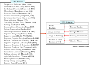
Source 1: Urban Improvement Trust, Sikar

Similar content being viewed by others

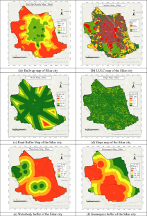
Identification of optimal locations for green space initiatives through GIS-based multi-criteria analysis and the analytical hierarchy process

Analysis of Urban Ecology Framework in Urban Green Spaces and Infrastructure Component

Assessing the morphological distribution of urban green spaces for the future sustainable greenery planning: a case study of Penang, Malaysia

Data availability.

The data shall be made available on reasonable request.

Abebe MT, Megento TL (2017) Urban green space development using GIS-based multicriteria analysis in Addis Ababa metropolis. Applied Geomatics 9:247–261

Article   Google Scholar  

Ahmed B, Kamruzzaman MD, Zhu X, Rahman MS, Choi K (2013) Simulating land cover changes and their impacts on land surface temperature in Dhaka, Bangladesh. Remote Sensing 5(11):5969–5998

Al-Ghorayeb A, Al-Shaar W, Elkordi A, Faour G, Al-Shaar M, Attalah Y (2023) Land suitability analysis for sustainable urban development: a case of Nabatiyeh Region in Lebanon. J 6(2):267–285

Google Scholar  

Anguluri R, Narayanan P (2017) Role of green space in urban planning: outlook towards smart cities. Urban for Urban Green 25:58–65

Bagheri M, Sulaiman WNA, Vaghefi N (2013) Application of geographic information system technique and analytical hierarchy process model for land-use suitability analysis on coastal area. J Coast Conserv 17:1–10

Bahadure S, Kotharkar R (2015) Assessing the sustainability of mixed use neighbourhoods through residents’ travel behaviour and perception: the case of Nagpur. India Sustainability 7(9):12164–12189

Bahadure S, Kotharkar R (2018) Framework for measuring sustainability of neighbourhoods in Nagpur, India. Build Environ 127:86–97

Beatley T (2000) Preserving biodiversity: challenges for planners. J Am Plann Assoc 66(1):5–20

Bibri SE, Krogstie J (2017) Smart sustainable cities of the future: an extensive interdisciplinary literature review. Sustain Cities Soc 31:183–212. https://doi.org/10.1016/j.scs.2017.02.016

Bolund P, Hunhammar S (1999) Ecosystem services in urban areas. Ecol Econ 29(2):293–301

Bunruamkaew K, Murayam Y (2011) Site suitability evaluation for ecotourism using GIS & AHP: a case study of Surat Thani province, Thailand. Procedia Soc Behav Sci 21:269–278

Chandio IA, Matori A-N, Lawal DU, Sabri S (2011) GIS-based land suitability analysis using AHP for public parks planning in Larkana City. Mod Appl Sci 5(4):177

Dağıstanlı C, Demirağ Turan İ, Dengiz O (2018) Evaluation of the suitability of sites for outdoor recreation using a multicriteria assessment model. Arab J Geosci. https://doi.org/10.1007/s12517-018-3856-0

Dawane V, Yatoo SA, Piplode S, Patidar SK, Joshi V, Muhammad A, Agarwal S, Kumar P (2023) Importance of climatological contributions in the green infrastructure designs, sustainable city planning towards better urban settlement. Climate Change and Urban Environment Sustainability. Springer Nature Singapore, Singapore, pp 47–79

Chapter   Google Scholar  

Fairbrass AJ, Jones K, McIntosh ALS, Yao Z, Malki-Epshtein L, Bell SJ (2018) Green infrastructure for London: a review of the evidence. https://discovery.ucl.ac.uk/id/eprint/10053788/1/ucl-green-infrastructure-for-london.pdf

Gelan E (2021) GIS-based multicriteria analysis for sustainable urban green spaces planning in emerging towns of Ethiopia: the case of Sululta town. Environ Syst Res 10(1):1–14

Goddard MA, Dougill AJ, Benton TG (2010) Scaling up from gardens: biodiversity conservation in urban environments. Trends Ecol Evol 25(2):90–98

Gül A, Örücü MK, Karaca Ö (2006) An approach for recreation suitability analysis to recreation planning in Gölcük Nature Park. Environ Manage 37:606–625

Haaland C, van den Bosch CK (2015) Challenges and strategies for urban greenspace planning in cities undergoing densification: a review. Urban Forest Urban Green 14(4):760–771. https://doi.org/10.1016/j.ufug.2015.07.009

Hailemariam B (2021) Suitable site selection for urban green space development using geographic information system and remote sensing based on multi criterion analysis. Int J Human Capital Urban Manag 6(1):97–110

Hörnsten L, Fredman P (2000) On the distance to recreational forests in Sweden. Landsc Urban Plan 51(1):1–10

Jabir K, DasS A (2014) Evaluation of recreational site selection and the prospects of recreational. Int J Environ Sci 3(1):17–21

Kamble T, Bahadure S, Punglia S (2022) Availability and accessibility of urban green spaces in a high-density city: the case of Raipur. India Prof Geogr 74(2):290–303. https://doi.org/10.1080/00330124.2021.2007495

Kaveh M, Kaveh M, Mesgari MS, Paland RS (2020) Multiple criteria decision-making for hospital location-allocation based on improved genetic algorithm. Applied Geomatics 12(3):291–306. https://doi.org/10.1007/s12518-020-00297-5

Kerstin M (2006) Food and Agriculture Organization of the United Nations (FAO). Oxford University Press. https://doi.org/10.1093/law:epil/9780199231690/e462

Book   Google Scholar  

Kienast F, Degenhardt B, Weilenmann B, Wäger Y, Buchecker M (2012) GIS-assisted mapping of landscape suitability for nearby recreation. Landsc Urban Plan 105(4):385–399

Kumar M, Shaikh VR (2012) Site suitability analysis for urban development using GIS based multicriteria evaluation technique. J Indian Soc Remote Sens 41(2):417–424. https://doi.org/10.1007/s12524-012-0221-8

Lahoti S, Kefi M, Lahoti A, Saito O (2019) Mapping methodology of public urban green spaces using GIS: an example of Nagpur City. India Sustain 11(7):2166

Lashari Z, Mangi MY, Sahito N, Brohi S, Meghwar S, Khokhar QUD (2017) Land suitability analysis for public parks using the GIS application. Sindh Univ Res j: SURJ (Science Series) 49(3):505–512

Li et al (2018) Urban Green Space Suitability Evaluation Based on the AHP-CV Combined Weight Method: A Case Study of Fuping County, China. https://www.mdpi.com/2071-1050/10/8/2656

Li C, Zhang T, Wang X, Lian Z (2022) Site selection of urban parks based on fuzzy-analytic hierarchy process (F-AHP): a case study of Nanjing, China. Int J Environ Res Public Health 19(20):13159

Mahdavi A, Niknejad M (2014) Site suitability evaluation for ecotourism using MCDM methods and GIS: case study-Lorestan province. Iran J Biodivers Environ Sci 4(6):425–437

Makkulawu AR, Santoso I, Mustaniroh SA (2023) Exploring the Potential and Benefits of AHP and GIS Integration for Informed Decision-Making: A Literature Review. Ingénierie Des Systèmes d’Information, 28(6). https://search.ebscohost.com/login.aspx?direct=true&profile=ehost&scope=site&authtype=crawler&jrnl=16331311&AN=174571219&h=g06EIYNlKcZX%2BiLnMyVXhjRnO4IclJNfMO0fMIy2giffdFOakiXt2JzVMqBcIQtBnfxTwtBCGW2fIVUlreJTrg%3D%3D&crl=c

Malczewski J (1999) GIS and multicriteria decision analysis. John Wiley & Sons

Malczewski J (2004) GIS-based land-use suitability analysis: a critical overview. Prog Plan 62(1):3–65. https://doi.org/10.1016/j.progress.2003.09.002

Malmir M, Zarkesh MMK, Monavari SM, Jozi SA, Sharifi E (2016) Analysis of land suitability for urban development in Ahwaz County in southwestern Iran using fuzzy logic and analytic network process (ANP). Environ Monit Assess 188:1–23

Manlun Y (2003) Suitability Analysis of Urban Green Space System Based on GIS

McConnachie MM, Shackleton CM (2010) Public green space inequality in small towns in South Africa. Habitat Int 34(2):244–248

Miller RW, Hauer RJ, Werner LP (2015) Urban forestry: planning and managing urban greenspaces. Waveland press

Moghadam HS, Helbich M (2013) Spatiotemporal urbanization processes in the megacity of Mumbai, India: a markov chains-cellular automata urban growth model. Appl Geogr 40:140–149

Mohammad M, Sahebgharani A, Malekipour E (2013) Urban growth simulation through cellular automata (CA), analytic hierarchy process (AHP) and GIS; case study of 8th and 12th municipal districts of Isfahan. Geographia Technica 8(2):57–70

Morckel V (2017) Using suitability analysis to select and prioritize naturalization efforts in legacy cities: an example from Flint, Michigan. Urban Forestry & Urban Greening 27:343–351

Nesticò A, Passaro R, Maselli G, Somma P (2022) Multicriteria methods for the optimal localization of urban green areas. J Clean Prod 374:133690

Niemelä J, Saarela S-R, Söderman T, Kopperoinen L, Yli-Pelkonen V, Väre S, Kotze DJ (2010) Using the ecosystem services approach for better planning and conservation of urban green spaces: a Finland case study. Biodivers Conserv 19(11):3225–3243. https://doi.org/10.1007/s10531-010-9888-8

Oliveira S, Andrade H, Vaz T (2011) The cooling effect of green spaces as a contribution to the mitigation of urban heat: a case study in Lisbon. Build Environ 46(11):2186–2194

Pantalone S (2010) Creating the urban Forest: Suitability analysis for green space in the City of Boston. Tufts University, USGS Land Cover Institute

Pareta K (2013) Remote sensing and GIS based site suitability analysis for tourism development. Int J Adv Res Eng Appl Sci 2(5):43–58

Piran H, Maleknia R, Akbari H, Soosani J, Karami O (2013) Site selection for local forest park using analytic hierarchy process and geographic information system (case study: Badreh County). Int Res J Appl Basic Sci 6(7):930–935

Pokhrel S (2019) Green space suitability evaluation for urban resilience: an analysis of Kathmandu Metropolitan city Nepal. Environ Res Commun 1(10):105003

Pramanik MK (2016) Site suitability analysis for agricultural land use of Darjeeling district using AHP and GIS techniques. Modeling Earth Syst Environ 2:1–22

Ramya S, Devadas V (2019) Integration of GIS, AHP and TOPSIS in evaluating suitable locations for industrial development: a case of Tehri Garhwal district, Uttarakhand. India J Clean Prod 238:117872. https://doi.org/10.1016/j.jclepro.2019.117872

Randrup TB, Persson B (2009) Public green spaces in the Nordic countries: development of a new strategic management regime. Urban Forest Urban Green 8(1):31–40

Saaty TL (1980a) The analytic hierarchy process Mcgraw Hill. Agricultural Economics Review, New York, p 70

Saaty TL (1980b) The analytic hierarchy process. Mcgrawhill international, New York

Sangwan A, Saraswat A, Kumar N, Pipralia S, Kumar A (2022) Urban green spaces prospects and retrospect’s. IntechOpen. https://doi.org/10.5772/intechopen.102857

Sangwan A, Choudhary S, Anand V, Kumar N, Kumar A, Jat MK, Ahmed R (2023a) A mathematical model for temperature-reducing potential of urban greenspaces. Earth Sci Inf 16(4):4199–4211. https://doi.org/10.1007/s12145-023-01166-6

Sangwan A, Kumar N, Kumar A (2023b) Amorphous nature of green spaces in Indian urban planning. Int Rev Spat Plan Sustain Dev 11(1):208–225

Sangwan A, Kumar N, Kumar A (2023c) Defining the urban greenspaces in the Indian context. Archit Urban Plan 19(1):76–92

Santosh C, Krishnaiah C, Deshbhandari PG (2018) Site suitability analysis for urban development using GIS based multicriteria evaluation technique: a case study in Chikodi Taluk, Belagavi District, Karnataka, India. IOP Conf Ser: Earth Environ Sci 169(1):012017

Sharma et al (2022) Urban Green Space Planning and Development in Urban Cities Using Geospatial Technology: A Case Study of Noida. https://sciendo.com/article/10.2478/jlecol-2022-0002

Stessens P, Canters F, Huysmans M, Khan AZ (2020) Urban green space qualities: an integrated approach towards GIS-based assessment reflecting user perception. Land Use Policy 91:104319. https://doi.org/10.1016/j.landusepol.2019.104319

Tahmasebi E, Jalali M, Gharehghashlo M, Nicknamfar M, Bahmanpour H (2014) Urban park site selection at local scale by using geographic information system (GIS) and analytic hierarchy process (AHP). Eur J Exp Biol 4(3):357–365

Tian L, Ge B, Li Y (2017) Impacts of state-led and bottom-up urbanization on land use change in the peri-urban areas of Shanghai: Planned growth or uncontrolled sprawl? Cities 60:476–486. https://doi.org/10.1016/j.cities.2016.01.002

Tsiko RG, Haile TS (2011) Integrating geographical information systems, fuzzy logic and analytical hierarchy process in modelling optimum sites for locating water reservoirs. A case study of the Debub District in Eritrea. Water 3(1):254–290

Ustaoglu E, Aydınoglu AC (2020) Site suitability analysis for green space development of Pendik district (Turkey). Urban Forest Urban Green 47:126542

Uy PD, Nakagoshi N (2008) Application of land suitability analysis and landscape ecology to urban greenspace planning in Hanoi, Vietnam. Urban Forest Urban Green 7(1):25–40

Wahdaty HM (2019) IT Based Land Suitability Modeling for Urban Development Using GIS: A Case Study of Kabul City, Afghanistan. J Int J Sci Res (IJSR) 8(9):235–240. https://paper.researchbib.com/view/paper/296406

Wu J (2014) Urban ecology and sustainability: The state-of-the-science and future directions. Landsc Urban Plan 125:209–221

Yang F, Zeng G, Du C, Tang L, Zhou J, Li Z (2008) Spatial analyzing system for urban land-use management based on GIS and multicriteria assessment modeling. Prog Nat Sci 18(10):1279–1284. https://doi.org/10.1016/j.pnsc.2008.05.007

Yang J, Liu Y, Wang S (2007) An overview of the methods of GIS-based land-use suitability analysis. In: P Gong, Y Liu (Eds.). In: SPIE Proceedings. SPIE. https://doi.org/10.1117/12.765488

Zhang X, Fang C, Wang Z, Ma H (2013) Urban construction land suitability evaluation based on improved multicriteria evaluation based on GIS (MCE-GIS): case of New Hefei City, China. Chin Geogra Sci 23:740–753

Ziyari YA, Sattari MH (2014) Site selection and prioritize urban parks and green spaces (case study: district 22 of Tehran municipality). Tech J Eng Appl Sci 4(4):230–243

Download references

The authors declare that no funds, grants, or other support were received during the preparation of this manuscript.

Author information

Authors and affiliations.

Department of Architecture and Planning, MNIT Jaipur, Jaipur, Rajasthan, 302017, India

Akanksha Sangwan, Nand Kumar & Mahesh Kumar Jat

Department of Civil Engineering, MNIT Jaipur, Jaipur, Rajasthan, 302017, India

Vijay Ananad

Department of Architecture and Planning, NIT Hamirpur, Hamirpur, Himachal Pradesh, 177055, India

Ashwani Kumar

Department of Geography and Disaster Management, School of Earth and Environmental Sciences, University of Kashmir, Srinagar, 190006, India

Rayees Ahmed

You can also search for this author in PubMed   Google Scholar

Contributions

Conceptualization, A.S.; methodology, A.S., software: A.S., V.A.; investigation, A.S.,; resources, N.K., A.K and M.K; data curation, A.S.; writing—original draft preparation, A.S.; Draft review: A.S., V.A.,Revision review: A.S., V.A.,: R.R. Final writing—review and editing, A.S.,V.A.; supervision, N.K., A.K and M.K. All authors have read and agreed to the published version of the manuscript.

Corresponding author

Correspondence to Akanksha Sangwan .

Ethics declarations

Conflict of interest.

The authors declare no competing interests.

Additional information

Publisher's note.

Springer Nature remains neutral with regard to jurisdictional claims in published maps and institutional affiliations.

Rights and permissions

Springer Nature or its licensor (e.g. a society or other partner) holds exclusive rights to this article under a publishing agreement with the author(s) or other rightsholder(s); author self-archiving of the accepted manuscript version of this article is solely governed by the terms of such publishing agreement and applicable law.

Reprints and permissions

About this article

Sangwan, A., Ananad, V., Kumar, N. et al. Development of site suitability framework for urban greenspace: a case study of Sikar city, Rajasthan, India. Environ Earth Sci 83 , 634 (2024). https://doi.org/10.1007/s12665-024-11898-3

Download citation

Received : 15 September 2023

Accepted : 30 September 2024

Published : 11 November 2024

DOI : https://doi.org/10.1007/s12665-024-11898-3

Share this article

Anyone you share the following link with will be able to read this content:

Sorry, a shareable link is not currently available for this article.

Provided by the Springer Nature SharedIt content-sharing initiative

• Site suitability
• Urban planning
• Find a journal
• Publish with us
• Track your research